Computer Vision Assignment 3

This is the third assignment for the Computer Vision (CSE-527) course from Fall 19 at Stony Brook University. As part of this assignment I learnt about scene recognition using multiple methods like tiny images, nearest neighbor classification and using bag of quantized local features with linear SVM.

NOTE: Using SIFT in OpenCV 3.x.x

Use the notes from the start of this post.

Bag of words models are a popular technique for image classification inspired by models used in natural language processing. The model ignores or downplays word arrangement (spatial information in the image) and classifies based on a histogram of the frequency of visual words. The visual word “vocabulary” is established by clustering a large corpus of local features.

For this homework we implement a basic bag of words model. We classify scenes into one of 16 categories by training and testing on the 16 scene database (introduced in Lazebnik et al. 2006, although built on top of previously published datasets). Lazebnik et al. 2006 is a great paper to read, although we will implemented the baseline method the paper discusses (equivalent to the zero level pyramid) and not the more sophisticated spatial pyramid. For an excellent survey of pre-deep-learning feature encoding methods for bag of words models, see Chatfield et al, 2011.

We implemented 2 different image representations: tiny images and bags of SIFT features, and 2 different classification techniques: nearest neighbor and linear SVM.

Dataset

---

The starter code trains on 150 and tests on 50 images from each category (i.e. 2400 training examples total and 800 test cases total). In a real research paper, one would be expected to test performance on random splits of the data into training and test sets, but the starter code does not do this to ease debugging.

Save the dataset(click me) into your working folder. Under your root folder, there should be a folder named “data” containing the images.

Starter Code

---

Below is some starter code which randomly guesses the category of every test image and achieves about 6.25% accuracy (1 out of 16 guesses is correct).

# import packages here
import cv2
import numpy as np
import matplotlib.pyplot as plt
import glob
import itertools
import time
import zipfile
import torch
import torchvision
import gc
import pickle
from sklearn import svm
from skimage import color
from skimage import io
from torch.utils.data import Dataset, DataLoader
from sklearn.neighbors import KNeighborsClassifier
from sklearn.cluster import KMeans
from sklearn.neighbors import NearestNeighbors
from sklearn.metrics import accuracy_score

from sklearn.svm import SVC
from sklearn.multiclass import OneVsRestClassifier

import random

from sklearn.metrics import confusion_matrix

print(cv2.__version__) # verify OpenCV version

3.4.2

Data Preparation

class_names = [name[13:] for name in glob.glob('./data/train/*')]
class_names = dict(zip(range(len(class_names)), class_names))
print("class_names: %s " % class_names)
n_train_samples_per_class = 150
n_test_samples_per_class = 50

def load_dataset(path, num_per_class=-1):
    data = []
    labels = []
    for id, class_name in class_names.items():
        print("Loading images from class: %s" % id)
        img_path_class = glob.glob(path + class_name + '/*.jpg')
        if num_per_class > 0:
            img_path_class = img_path_class[:num_per_class]
        labels.extend([id]*len(img_path_class))
        for filename in img_path_class:
            data.append(cv2.imread(filename, 0))
    return data, labels

# load training dataset
# train_data, train_label = load_dataset('./data/train/')
train_data, train_label = load_dataset('./data/train/', n_train_samples_per_class)
n_train = len(train_label)
print("n_train: %s" % n_train)

# load testing dataset
# test_data, test_label = load_dataset('./data/test/')
test_data, test_label = load_dataset('./data/test/', n_test_samples_per_class)
n_test = len(test_label)
print("n_test: %s" % n_test)

class_names: {0: 'LivingRoom', 1: 'Mountain', 2: 'OpenCountry', 3: 'Suburb', 4: 'Store', 5: 'Kitchen', 6: 'InsideCity', 7: 'Office', 8: 'TallBuilding', 9: 'Street', 10: 'Forest', 11: 'Industrial', 12: 'Highway', 13: 'Coast', 14: 'Flower', 15: 'Bedroom', 16: '_DS_Store'} 
Loading images from class: 0
Loading images from class: 1
Loading images from class: 2
Loading images from class: 3
Loading images from class: 4
Loading images from class: 5
Loading images from class: 6
Loading images from class: 7
Loading images from class: 8
Loading images from class: 9
Loading images from class: 10
Loading images from class: 11
Loading images from class: 12
Loading images from class: 13
Loading images from class: 14
Loading images from class: 15
Loading images from class: 16
n_train: 2400
Loading images from class: 0
Loading images from class: 1
Loading images from class: 2
Loading images from class: 3
Loading images from class: 4
Loading images from class: 5
Loading images from class: 6
Loading images from class: 7
Loading images from class: 8
Loading images from class: 9
Loading images from class: 10
Loading images from class: 11
Loading images from class: 12
Loading images from class: 13
Loading images from class: 14
Loading images from class: 15
Loading images from class: 16
n_test: 400

# As loading the data from the source for the first time is time consuming, so you can pkl or save the data in a compact way such that subsequent data loading is faster
# Save intermediate image data into disk
file = open('train.pkl','wb')
pickle.dump(train_data, file)
pickle.dump(train_label, file)
file.close()

file = open('test.pkl','wb')
pickle.dump(test_data, file)
pickle.dump(test_label, file)
file.close()

# Load intermediate image data from disk
file = open('train.pkl', 'rb')
train_data = pickle.load(file)
train_label = pickle.load(file)
file.close()

file = open('test.pkl', 'rb')
test_data = pickle.load(file)
test_label = pickle.load(file)
file.close()

print(len(train_data), len(train_label)) # Verify number of training samples
print(len(test_data), len(test_label))   # Verify number of testing samples

2400 2400
400 400

# plt.imshow(train_data[1], cmap='gray') # Verify image
img_new_size = (240, 240)

train_data = list(map(lambda x: cv2.resize(x, img_new_size), train_data))
train_data = np.stack(train_data)
train_label = np.array(train_label)

test_data = list(map(lambda x: cv2.resize(x, img_new_size), test_data))
test_data = np.stack(test_data)
test_label = np.array(test_label)

# Verify image
plt.imshow(cv2.resize(train_data[1], img_new_size), cmap='gray')
print(train_data[0].dtype)

uint8

n_train = len(train_label)
n_test = len(test_label)

# feature extraction
def extract_feat(raw_data):
    print(len(raw_data))
    feat_dim = 1000
    feat = np.zeros((len(raw_data), feat_dim), dtype=np.float32)
    for i in np.arange(feat.shape[0]):
        feat[i] = np.reshape(raw_data[i], (raw_data[i].size))[:feat_dim] # dummy implemtation
    print("feat",len(feat))
    
    return feat

train_feat = extract_feat(train_data)
test_feat = extract_feat(test_data)

# model training: take feature and label, return model
def train(X, Y):
    return 0 # dummy implementation

# prediction: take feature and model, return label
def predict(model, x):
    return np.random.randint(16) # dummy implementation

# evaluation
predictions = [-1]*len(test_feat)
for i in np.arange(n_test):
    predictions[i] = predict(None, test_feat[i])
    
accuracy = sum(np.array(predictions) == test_label) / float(n_test)

print("The accuracy of my dummy model is {:.2f}%".format(accuracy*100))

2400
feat 2400
400
feat 400
The accuracy of my dummy model is 5.75%

Problem 1: Tiny Image Representation + Nearest Neighbor Classifier

We start by implementing the tiny image representation and the nearest neighbor classifier. They are easy to understand, easy to implement, and run very quickly for our experimental setup.

The “tiny image” feature is one of the simplest possible image representations. One simply resizes each image to a small, fixed resolution. You are required to resize the image to 16x16. It works slightly better if the tiny image is made to have zero mean and unit length (normalization). This is not a particularly good representation, because it discards all of the high frequency image content and is not especially invariant to spatial or brightness shifts. We are using tiny images simply as a baseline.

The nearest neighbor classifier is equally simple to understand. When tasked with classifying a test feature into a particular category, one simply finds the “nearest” training example (L2 distance is a sufficient metric) and assigns the label of that nearest training example to the test example. The nearest neighbor classifier has many desirable features — it requires no training, it can learn arbitrarily complex decision boundaries, and it trivially supports multiclass problems. It is quite vulnerable to training noise, though, which can be alleviated by voting based on the K nearest neighbors (but you are not required to do so). Nearest neighbor classifiers also suffer as the feature dimensionality increases, because the classifier has no mechanism to learn which dimensions are irrelevant for the decision.

Report your classification accuracy on the test sets and time consumption.

Hints:

• Use cv2.resize() to resize the images;
• Use NearestNeighbors in Sklearn as your nearest neighbor classifier.

start_time = time.time()
# Convert training and test data into tiny images
tiny_image_size = (16, 16)
train_data_tiny = list(map(lambda x: cv2.resize(x, tiny_image_size, interpolation=cv2.INTER_AREA).flatten(), train_data))
train_data_tiny = np.stack(train_data_tiny)
test_data_tiny = list(map(lambda x: cv2.resize(x, tiny_image_size, interpolation=cv2.INTER_AREA).flatten(), test_data))
test_data_tiny = np.stack(test_data_tiny)

# Prepare Nearest Neighbor Classifier
n_neighbors = 1
clf = NearestNeighbors(n_neighbors, metric='l2')

# Fit training data
neighbors = clf.fit(train_data_tiny)

# Make prediction
distances, nearest_neighbors = neighbors.kneighbors(test_data_tiny)

# print(train_label, len(train_label))
# print(test_label, len(test_label))
# print(nearest_neighbors, len(nearest_neighbors))
# print(distances)
pred1 = list(map(lambda x: train_label[x], nearest_neighbors))
# print(predicted_labels)

total_elapsed_time = time.time() - start_time
print('Time to complete task: {}s'.format(total_elapsed_time))
print("The accuracy of NearestNeighbors classigier is {:.2f}%".format(accuracy_score(test_label, pred1)*100))

Time to complete task: 0.678107500076294s
The accuracy of NearestNeighbors classigier is 22.75%

Problem 2: Bag of SIFT Representation + Nearest Neighbor Classifer

After you have implemented a baseline scene recognition pipeline it is time to move on to a more sophisticated image representation — bags of quantized SIFT features. Before we can represent our training and testing images as bag of feature histograms, we first need to establish a vocabulary of visual words. We will form this vocabulary by sampling many local features from our training set (10’s or 100’s of thousands) and then cluster them with k-means. The number of k-means clusters is the size of our vocabulary and the size of our features. For example, you might start by clustering many SIFT descriptors into k=50 clusters. This partitions the continuous, 128 dimensional SIFT feature space into 50 regions. For any new SIFT feature we observe, we can figure out which region it belongs to as long as we save the centroids of our original clusters. Those centroids are our visual word vocabulary. Because it can be slow to sample and cluster many local features, the starter code saves the cluster centroids and avoids recomputing them on future runs.

Now we are ready to represent our training and testing images as histograms of visual words. For each image we will densely sample many SIFT descriptors. Instead of storing hundreds of SIFT descriptors, we simply count how many SIFT descriptors fall into each cluster in our visual word vocabulary. This is done by finding the nearest neighbor k-means centroid for every SIFT feature. Thus, if we have a vocabulary of 50 visual words, and we detect 220 distinct SIFT features in an image, our bag of SIFT representation will be a histogram of 50 dimensions where each bin counts how many times a SIFT descriptor was assigned to that cluster. The total of all the bin-counts is 220. The histogram should be normalized so that image size does not dramatically change the bag of features magnitude.

After you obtain the Bag of SIFT feature representation of the images, you have to train a KNN classifier in the Bag of SIFT feature space and report your test set accuracy and time consumption.

Note:

• Instead of using SIFT to detect invariant keypoints which is time-consuming, you are recommended to densely sample keypoints in a grid with certain step size (sampling density) and scale.
• There are many design decisions and free parameters for the bag of SIFT representation (number of clusters, sampling density, sampling scales, SIFT parameters, etc.) so accuracy might vary from 50% to 60%.
• Indicate clearly the parameters you use along with the prediction accuracy on test set and time consumption.

Hints:

• Use KMeans in Sklearn to do clustering and find the nearest cluster centroid for each SIFT feature;
• Use cv2.xfeatures2d.SIFT_create() to create a SIFT object;
• Use sift.compute() to compute SIFT descriptors given densely sampled keypoints (cv2.Keypoint).
• Be mindful of RAM usage. Try to make the code more memory efficient, otherwise it could easily exceed RAM limits in Colab, at which point your session will crash.
• If your RAM is going to run out of space, use gc.collect() for the garbage collector to collect unused objects in memory to free some space.
• Store data or features as NumPy arrays instead of lists. Computation on NumPy arrays is much more efficient than lists.

# 240x240
# train_data
# test_data
start_time = time.time()

# Prepare images with set keypoints and descriptors
size = [240, 240]
step = 20
scale = 8
keypoints = [cv2.KeyPoint(i, j, scale) for i in range(step, size[0], step) for j in range(step, size[1], step)]
print('Step size and scale for keypoints: {} and {}'.format(step, scale))
print('Numer of keypoints per image {}'.format(len(keypoints)))
# print(keypoints)

descriptors_start_time = time.time()
sift = cv2.xfeatures2d.SIFT_create()
descriptors = []
for image in train_data:
  kp, des = sift.compute(image, keypoints)
  descriptors.extend(des)
#   print(des)
descriptors_elapsed_time = time.time() - descriptors_start_time
print('{} descriptors across all images computed in {}s'.format(len(descriptors), descriptors_elapsed_time))

# Calculate the K-Means of all descriptors
kmeans_start_time = time.time()
num_clusters=64
kmeansclf = KMeans(n_clusters=num_clusters, random_state=0)
kmeans = kmeansclf.fit(descriptors)
kmeans_elapsed_time = time.time() - kmeans_start_time
print('Total time to calculate k-means with {} clusters: {}s'.format(num_clusters, kmeans_elapsed_time))

# Calculate bag of histograms
histograms_start_time = time.time()
image_histograms = []
for image in train_data:
  kp, des = sift.compute(image, keypoints)
  histogram = np.zeros(num_clusters)
  number_keypoints = np.size(kp)
  for d in des:
    index = kmeans.predict(des)
    histogram[index] += 1/number_keypoints
    
  image_histograms.append(histogram)

histograms_elapsed_time = time.time() - histograms_start_time
print('Total time to build nomalized histogram representation of all {} images: {}s'.format(len(image_histograms), histograms_elapsed_time))

# Train K-Neighbors Classifer on Bag of Histograms
train_start_time = time.time()
k=30
neigh = KNeighborsClassifier(n_neighbors=k, weights='distance')
neigh.fit(np.array(image_histograms), train_label)
train_elapsed_time = time.time() - train_start_time
print('Total time to train K-Neighbors Classifier on {} histograms: {}s'.format(len(image_histograms), train_elapsed_time))

# Prepare Test data and predict labels
prediction_start_time = time.time()
test_image_histograms = []
for image in test_data:
  kp, des = sift.compute(image, keypoints)
  
  histogram = np.zeros(num_clusters)
  number_keypoints = np.size(kp)
  for d in des:
    index = kmeans.predict(des)
    histogram[index] += 1/number_keypoints
    
  test_image_histograms.append(histogram)

pred2 = neigh.predict(test_image_histograms)
prediction_elapsed_time = time.time() - prediction_start_time
print('Total time to prepare {} test image histograms and predict labels: {}s'.format(len(test_image_histograms), prediction_elapsed_time))

total_elapsed_time = time.time() - start_time
print('Time to complete task: {}s'.format(total_elapsed_time))
print("The accuracy of KNN classigier on Bag of SIFT Features is {:.2f}%".format(accuracy_score(test_label, pred2)*100))

Step size and scale for keypoints: 20 and 8
Numer of keypoints per image 121
290400 descriptors across all images computed in 19.26657009124756s
Total time to calculate k-means with 64 clusters: 723.0350425243378s
Total time to build nomalized histogram representation of all 2400 images: 268.4476327896118s
Total time to train K-Neighbors Classifier on 2400 histograms: 0.014222860336303711s
Total time to prepare 400 test image histograms and predict labels: 47.27513647079468s
Time to complete task: 1058.041999578476s
The accuracy of KNN classigier on Bag of SIFT Features is 48.25%

Problem 3.a: Bag of SIFT Representation + one-vs-all SVMs

The last task is to train one-vs-all linear SVMS to operate in the bag of SIFT feature space. Linear classifiers are one of the simplest possible learning models. The feature space is partitioned by a learned hyperplane and test cases are categorized based on which side of that hyperplane they fall on. Despite this model being far less expressive than the nearest neighbor classifier, it will often perform better.

You do not have to implement the support vector machine. However, linear classifiers are inherently binary and we have a 16-way classification problem (the library has handled it for you). To decide which of 16 categories a test case belongs to, you will train 16 binary, one-vs-all SVMs. One-vs-all means that each classifier will be trained to recognize ‘forest’ vs ‘non-forest’, ‘kitchen’ vs ‘non-kitchen’, etc. All 16 classifiers will be evaluated on each test case and the classifier which is most confidently positive “wins”. E.g. if the ‘kitchen’ classifier returns a score of -0.2 (where 0 is on the decision boundary), and the ‘forest’ classifier returns a score of -0.3, and all of the other classifiers are even more negative, the test case would be classified as a kitchen even though none of the classifiers put the test case on the positive side of the decision boundary. When learning an SVM, you have a free parameter $\lambda$ (lambda) which controls how strongly regularized the model is. Your accuracy will be very sensitive to $\lambda$, so be sure to try many values.

Indicate clearly the parameters you use along with the prediction accuracy on test set and time consumption.

You can generate class prediction for the images in test2 folder using your best model.

Hints:

• Use SVM in Sklearn (recommended) or OpenCV to do training and prediction.

def onevsrest_simple_svc(image_histograms, train_label, test_image_histograms, test_label, train_lambda=0.008):
  classif = SVC(C=train_lambda, kernel='linear', probability=True, random_state=42)
  classif.fit(np.array(image_histograms), train_label)
  pred3 = classif.predict(test_image_histograms)
  accuracy = accuracy_score(test_label, pred3)*100
  return pred3, accuracy
  
# for train_lambda in np.arange(0.09, 0.21, 0.01):
train_lambda = 0.11
print('Regularization Factor: {}'.format(train_lambda))
start_time = time.time()
# print(len(image_histograms), train_label, len(test_image_histograms), test_label, train_lambda)
pred3, accuracy = onevsrest_simple_svc(image_histograms, train_label, test_image_histograms, test_label, train_lambda)
elapsed_time = time.time() - start_time
print("The accuracy of SVC classifier on Bag of SIFT Features computed in {:.2f}s is {:.2f}%".format(elapsed_time, accuracy))

Regularization Factor: 0.11
The accuracy of SVC classifier on Bag of SIFT Features computed in 1.91s is 52.50%

# PREDICTION ON TEST2 IMAGES
test2_data = []
test2_image_file_names = glob.glob('./data/test2/*.jpg')

for filename in test2_image_file_names:
  test2_data.append(cv2.imread(filename, 0))
  
test2_image_histograms = []
for image in test2_data:
  kp, des = sift.compute(image, keypoints)
  
  histogram = np.zeros(num_clusters)
  number_keypoints = np.size(kp)
  for d in des:
    index = kmeans.predict(des)
    histogram[index] += 1/number_keypoints
    
  test2_image_histograms.append(histogram)

train_lambda = 0.11
classif = SVC(C=train_lambda, kernel='linear', probability=True, random_state=42)
classif.fit(np.array(image_histograms), train_label)
test2_pred = classif.predict(test2_image_histograms)

flush = ['Name Class_id\n']
for index, filename in enumerate(test2_image_file_names):
  name = filename[13:-4]
  flush.append('{} {}\n'.format(name, test2_pred[index]))

# print(flush)
f = open("Acharya_Narayan_112734365_Pred.txt", "w")
f.writelines(flush)
f.close()

Problem 3.b

Repeat the evaluation above for different sizes of training sets and draw a plot to show how the size of the training set affects test performace. Do this for training set sizes of 800, 1200, 1600, 2000, 2200, and 2300 images. Randomly sample the images from the original training set and evaluate accuracy. Repeat this process 10 times for each training set size and report the average prediction accuracy. How does performance variability change with training set size? How does performance change? Give reason for your observations.

NOTE:

We use the same lambda value of 0.11 that we found the best results for in Q3a for these evaluations.

trials = 10
training_set_sizes = [800, 1200, 1600, 2000, 2200, 2300]
for sample_size in training_set_sizes:
  start_time = time.time()
  accuracies = []
  for i in range(0, trials):
    sampled_train_histograms, sampled_train_labels = zip(*random.sample(list(zip(image_histograms, train_label)), sample_size))
    predictions, accuracy = onevsrest_simple_svc(sampled_train_histograms, sampled_train_labels, test_image_histograms, test_label, train_lambda=0.11)
    accuracies.append(accuracy)
  
  elapsed_time = time.time() - start_time
  print("""Accuracies for sample size {} computed in {:.2f}s: {}""".format(sample_size, elapsed_time, ["%.2f" % member for member in accuracies]))
  mean_accuracy = sum(accuracies) / len(accuracies)
  print("""The mean accuracy of One-Vs-All classigier on Bag of SIFT Features in
          {} trials and {} samples: {:.2f}%""".format(trials, sample_size, mean_accuracy))

Accuracies for sample size 800 computed in 3.49s: ['45.25', '47.50', '49.00', '42.75', '45.25', '48.25', '48.00', '48.25', '46.00', '46.50']
The mean accuracy of One-Vs-All classigier on Bag of SIFT Features in
          10 trials and 800 samples: 46.67%
Accuracies for sample size 1200 computed in 6.45s: ['47.00', '46.75', '44.25', '48.00', '50.75', '48.00', '47.25', '45.75', '47.25', '48.75']
The mean accuracy of One-Vs-All classigier on Bag of SIFT Features in
          10 trials and 1200 samples: 47.38%
Accuracies for sample size 1600 computed in 10.13s: ['47.00', '48.50', '50.00', '48.25', '49.75', '48.25', '49.75', '47.25', '48.75', '47.50']
The mean accuracy of One-Vs-All classigier on Bag of SIFT Features in
          10 trials and 1600 samples: 48.50%
Accuracies for sample size 2000 computed in 14.41s: ['49.50', '48.25', '51.50', '52.25', '52.00', '48.50', '49.75', '52.75', '50.50', '50.25']
The mean accuracy of One-Vs-All classigier on Bag of SIFT Features in
          10 trials and 2000 samples: 50.52%
Accuracies for sample size 2200 computed in 16.89s: ['50.00', '51.00', '49.00', '50.50', '49.75', '50.50', '50.50', '52.75', '48.50', '52.25']
The mean accuracy of One-Vs-All classigier on Bag of SIFT Features in
          10 trials and 2200 samples: 50.48%
Accuracies for sample size 2300 computed in 18.11s: ['52.50', '51.25', '50.75', '50.50', '53.25', '52.50', '51.75', '50.75', '50.50', '51.00']
The mean accuracy of One-Vs-All classigier on Bag of SIFT Features in
          10 trials and 2300 samples: 51.48%

Performance in terms of accuracy:

From the above numbers one can make out that as we increase the training set size there is steady rise in accuracy, from ~46% to ~51%. This is expected as we train with more samples we will be better equipped to classify all classes. Also, given that we randomly chose samples from our training set, it is quite possible that samples with a smaller training set size did not have enough (or maybe did not have any) examples for each(or any one) of the classes to be classified.

Performance in terms of time:

Time to train and predict also grew steadily from ~3s for 800 training set size to ~17s for the 2300 training set size. This too is expected as we require to fit our model over more examples as training set size increases.

Extra Note:

One thing to note here is that, not reflected in the output above, is that for training set sizes that are close to each other, like 2200 and 2300, we need not always get 2300 to perform better than 2200 in terms of mean accuracy over n number of trials. This is because these numbers are pretty close(keeping in mind that our total training size is 2400) and the randomness involved while choosing the samples might offset the accuracy based on what samples are chosen.

Performance Report

---

Please report the performance of the following combinations in the given order in terms of the time consumed and classification accuracy. Describe your algorithm, any decisions you made to write your algorithm in your particular way, and how different choices you made affect it. Compute and draw a (normalized) confusion matrix, and discuss where the method performs best and worse for each of the combination. Here is an example of how to compute confusion matrix.

1st: Tiny images representation and nearest neighbor classifier (accuracy of about 18-25%).
2nd: Bag of SIFT representation and nearest neighbor - classifier (accuracy of about 40-50%).
3rd: Bag of SIFT representation and linear SVM classifier (accuracy of about 50-70%).

NOTE: Below metrics are using Google Colab with

• NO Hardwarre acceleration
• RAM of 25.51GB (never maxed out under any configuration of tests)
• Disk Space of 48.97 GB.

1st: Tiny images representation and nearest neighbor classifier:

Max Accuracy: 22.75%
Computation Time: <1s

NOTES:

• Used the INTER_AREA metric for interpolation while resizing the images into tiny images. This performed better than the default as well as other interpolation techniques.
• Tried different metrics for finding the nearest neighbor like, minkowski with different p values. Default parameter, which is just l2 distance among the data points gave best results.

2nd: Bag of SIFT representation and nearest neighbor classifier:

Max Accuracy: 48.75%
Computation Time: ~1060s
Parameters Used:

• step: 20
• keypoint scale: 8
• K-Means clusters: 64
• KNN neighbors: 30

NOTES:

• Keypoints were placed at steps of 20 vertically and horizontally, with a scale of 8. This led to 121 descriptors per image and almost 290k descriptors across all images.
• Finding k-means with 64 clusters for above configuration took almost 720s.
• Packing keypoints more densely led to more descriptors but this led to more time spent finding the k-means clusters. Another configuration tried was with step=16 and scale=6 which led to almost 470k descriptors. Finding the k-means for so many descriptors was taking more than 30mins in Google Colab with no hardware acceleration applied.
• Constructing the histogram representation of each training image based on the descriptors was the second most time consuming task after the k-means. Took around 275s. Started with k=1 and k=5 for KNN, incrementing thereafter at intervals of 5. It was observed that higher values of k gave better results in terms of accuracy with hit to computation time. But returns diminished after a certain value. Finally settled on k=30 here.
• In the last step, we prepare our test images by constructing the histogram representation for all based on the k-means we calculated for the training images and then using the KNN Classifer trained above to predict the labels for our test images.
• Finally, we calculate the accuracy of the task and total computation time for the above steps which comes out to to be 48.75% and around 1060s respectively.

3rd: Bag of SIFT representation and linear SVM classifier

Max Accuracy: 52.50%
Computation Time: Given we use the same image histogram representations from Q2, the computation time will be equivalent to Q2. The time required to fit the SVC and predict is negligible compared to the time prep data like we did in Q2.
Parameters Used:

• lambda: 0.11

NOTES:

• Given sklearn now supports One-Vs-Rest classification for its SVCs, we directly use the SVC instead of OneVsRestClassifier with an underlying SVC.
• The only parameter to tweak here is the C(or lambda) which is the regularization constant responsible for controlling the error parameter.
• Initially incremented this parameter from 1 to 20, in increments of 1. Only to find that the finally accuracy did not budge much during consecutive trials and steadily kept dropping. Trying with values between 0 and 1 gave better results on the accuracy, just enough to cross the 50% mark. Max accuracy of 52.50 was achieved with lambda as 0.11.

def plot_confusion_matrix(cm, classes,
                          normalize=False,
                          title='Confusion matrix',
                          cmap=plt.cm.Blues):
    """
    This function prints and plots the confusion matrix.
    Normalization can be applied by setting `normalize=True`.
    """

    if normalize:
        cm = cm.astype('float') / cm.sum(axis=1)[:, np.newaxis]

    fig, ax = plt.subplots(figsize=(12,12))
    im = ax.imshow(cm, interpolation='nearest', cmap=cmap)
    ax.figure.colorbar(im, ax=ax)
    # We want to show all ticks...
    ax.set(xticks=np.arange(cm.shape[1]),
           yticks=np.arange(cm.shape[0]),
           xticklabels=classes, yticklabels=classes,
           title=title,
           ylabel='True label',
           xlabel='Predicted label')

    # Rotate the tick labels and set their alignment.
    plt.setp(ax.get_xticklabels(), rotation=45, ha="right", rotation_mode="anchor")

    # Loop over data dimensions and create text annotations.
    fmt = '.2f' if normalize else 'd'
    thresh = cm.max() / 2.
    for i in range(cm.shape[0]):
        for j in range(cm.shape[1]):
            ax.text(j, i, format(cm[i, j], fmt),
                    ha="center", va="center",
                    color="white" if cm[i, j] > thresh else "black")
    fig.tight_layout()
    return ax

# !pwd
c_names = []
if len(c_names) == 0:
  c_names = [name[13:] for name in glob.glob('./data/train/*')]

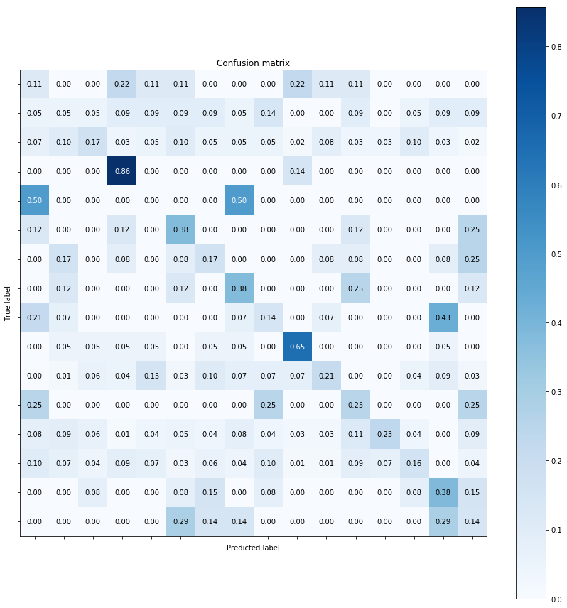
#First combination:
# Confusion matrix
cm1 = confusion_matrix(pred1, test_label)
plt.figure(figsize=(12,12))
plot_confusion_matrix(cm1, c_names, normalize=True)
plt.show()

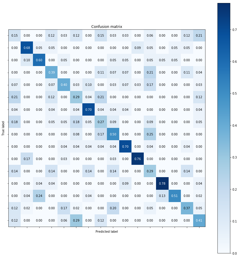
#Second combination:
# Confusion matrix
cm2 = confusion_matrix(pred2, test_label)
plt.figure(figsize=(12,12))
plot_confusion_matrix(cm2, c_names, normalize=True)
plt.show()

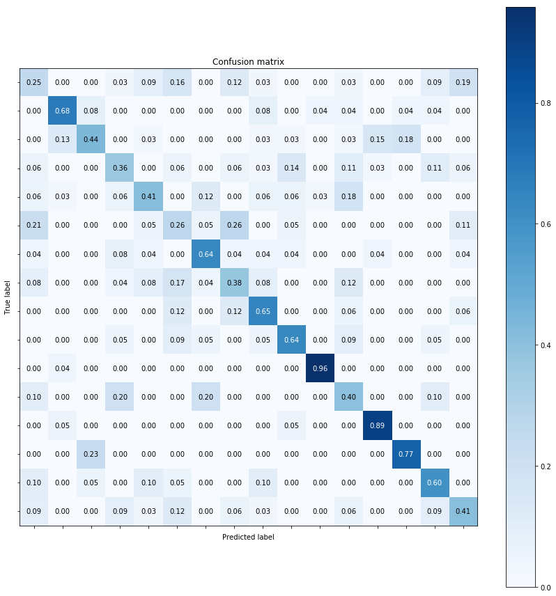
#Third combination:
# Confusion matrix
cm3 = confusion_matrix(pred3, test_label)
plt.figure(figsize=(12,12))
plot_confusion_matrix(cm3, c_names, normalize=True)
plt.show()

<Figure size 864x864 with 0 Axes>

<Figure size 864x864 with 0 Axes>

<Figure size 864x864 with 0 Axes>

NOTES ON ABOVE CONFUSION MATRICES:

• The confusion matrix is used to assess how accurately a particular classifer worked. To rephrase, calculate how many (or what percentage of times) was the true label equal to the predicted label of the class.
• The above can be easily visualized using a confusion matrix’s diagonal elements. These elements convey the number of time true labels were equal to predicted label. For a classifier with 100% accuracy we would see all the diagonal elements to be high while the non-diagonal elements to be exactly zero.
• The non-diagonal elements indicate how many times a particular label was ‘confused’ for another label. Say, for example, in our case how many times a forest was classified as a highway can be seen going to the row for forest and checking its column for highway. Ideally we would want this cell to be as close to zero as possible.
• With this understanding, it becomes easy to understand the confusion matrix of our 3 approaches.
  • For the tiny image and nearest neighbor based classifier we had a very low accuracy because our our predicted labels matched a very small percentage of the true labels of our testing images. This is reflected in the 1st confusion matrix above. Notice that the diagonal elements are not dark-shade of blue, indicating low values while the non-diagonal elements are a lighter shade of blue but instead should have been as close to white as possible.
  • For the Bag-Of-Histogram features with KNN Classifier, there was significant jump in the accuracy of the task. The 2nd confusion matrix also conveys the same. It has better diagonal elements values compared to the 1st.
  • For the Bag-Of-Histogram with an SVC, we had slightly better performance in terms of accuracy over the 2nd approach and we can a slightly better confusion matrix over the 2nd as well. Notice, in the 3rd confusion matrix above we got a normalize score of 0.96 and 0.89 for a couple of categories.

This wraps up assignment 3. You can find insights into assignments 1 and 2 by clicking here and here respectively.

Peace!