Computer Vision Assignment 2

15 minute read

This is the second assignment for the Computer Vision (CSE-527) course from Fall 19 at Stony Brook University. As part of this assignment I learnt to use SIFT features for scene matching and scene stitching. I also learnt about using Histogram of Gradients (HOG) as features for object recognition.

IMPORTANT NOTE: The images used in this assignment can be found here

NOTE: Using SIFT in OpenCV 3.x.x

Feature descriptors like SIFT and SURF are no longer included in OpenCV since version 3. This section provides instructions on how to use SIFT for those who use OpenCV 3.x.x. If you are using OpenCV 2.x.x then you are all set, please skip this section. Read this if you are curious about why SIFT is removed https://www.pyimagesearch.com/2015/07/16/where-did-sift-and-surf-go-in-opencv-3/.

However, if you want to use SIFT in your local machine, one simple way to use the OpenCV in-built function SIFT is to switch back to version 2.x.x, but if you want to keep using OpenCV 3.x.x, do the following:

uninstall your original OpenCV package
install opencv-contrib-python using pip: Please find detailed instructions at https://pypi.python.org/pypi/opencv-contrib-python

After you have your OpenCV set up, you should be able to use cv2.xfeatures2d.SIFT_create() to create a SIFT object, whose functions are listed at http://docs.opencv.org/3.0-beta/modules/xfeatures2d/doc/nonfree_features.html

Some Resources

In addition to the tutorial document, the following resources can come in handy:

http://opencv-python-tutroals.readthedocs.io/en/latest/py_tutorials/py_feature2d/py_matcher/py_matcher.html
http://docs.opencv.org/3.1.0/da/df5/tutorial_py_sift_intro.html
http://docs.opencv.org/3.0-beta/modules/xfeatures2d/doc/nonfree_features.html?highlight=sift#cv2.SIFT
http://docs.opencv.org/3.0-beta/doc/py_tutorials/py_imgproc/py_geometric_transformations/py_geometric_transformations.html

Lets get started with getting all the packages that we need imported and also verify the OpenCV version we use.

# import packages here
import cv2
import math
import numpy as np
import matplotlib.pyplot as plt
print(cv2.__version__) # verify OpenCV version

from os import listdir
from os.path import isfile, join
import random
from skimage.feature import hog
from skimage import data, exposure
from sklearn import svm
from sklearn.metrics import accuracy_score

3.4.2

Problem 1: Match transformed images using SIFT features

You will transform a given image, and match it back to the original image using SIFT keypoints.

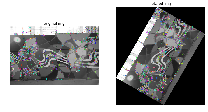
Step 1. Use the function from SIFT class to detect keypoints from the given image. Plot the image with keypoints scale and orientation overlaid.
Step 2. Rotate your image clockwise by 60 degrees with the cv2.warpAffine function. Extract SIFT keypoints for this rotated image and plot the rotated picture with keypoints scale and orientation overlaid just as in step 1.
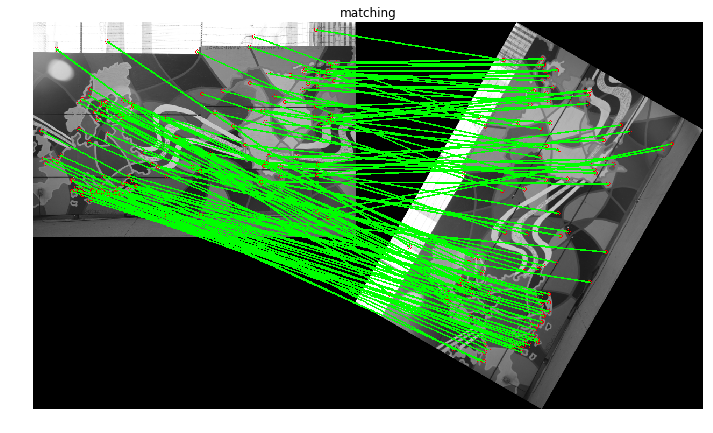
Step 3. Match the SIFT keypoints of the original image and the rotated imag using the knnMatch function in the cv2.BFMatcher class. Discard bad matches using the ratio test proposed by D.Lowe in the SIFT paper. Use 0.1 as the ratio in this homework. Note that this is for display purpose only. Draw the filtered good keypoint matches on the image and display it. The image you draw should have two images side by side with matching lines across them.
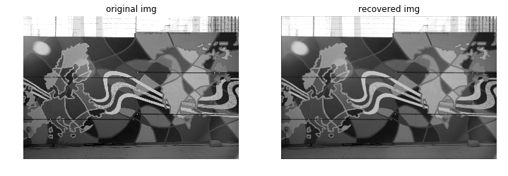
Step 4. Use the RANSAC algorithm to find the affine transformation from the rotated image to the original image. You are not required to implement the RANSAC algorithm yourself, instead you could use the cv2.findHomography function (set the 3rd parameter method to cv2.RANSAC) to compute the transformation matrix. Transform the rotated image back using this matrix and the cv2.warpPerspective function. Display the recovered image.
Step 5. You might have noticed that the rotated image from step 2 is cropped. Rotate the image without any cropping.

Hints: In case of too many matches in the output image, use the ratio of 0.1 to filter matches.

def drawMatches(img1, kp1, img2, kp2, matches):
    '''
    The TA's implementation of cv2.drawMatches as OpenCV 2.4.9
    does not have this function available but it's supported in
    OpenCV 3.0.0

    This function takes in two images with their associated 
    keypoints, as well as a list of DMatch data structure (matches) 
    that contains which keypoints matched in which images.

    An image will be produced where a montage is shown with
    the first image followed by the second image beside it.

    Keypoints are delineated with circles, while lines are connected
    between matching keypoints.

    img1,img2 - Grayscale images
    kp1,kp2 - Detected list of keypoints through any of the OpenCV keypoint 
              detection algorithms
    matches - A list of matches of corresponding keypoints through any
              OpenCV keypoint matching algorithm
    '''

    # Create a new output image that concatenates the two images together
    # (a.k.a) a montage
    rows1 = img1.shape[0]
    cols1 = img1.shape[1]
    rows2 = img2.shape[0]
    cols2 = img2.shape[1]

    # Create the output image
    # The rows of the output are the largest between the two images
    # and the columns are simply the sum of the two together
    # The intent is to make this a colour image, so make this 3 channels
    out = np.zeros((max([rows1,rows2]),cols1+cols2,3), dtype='uint8')

    # Place the first image to the left
    out[:rows1,:cols1] = np.dstack([img1, img1, img1])

    # Place the next image to the right of it
    out[:rows2,cols1:] = np.dstack([img2, img2, img2])

    # For each pair of points we have between both images
    # draw circles, then connect a line between them
    for mat in matches:

        # Get the matching keypoints for each of the images
        img1_idx = mat.queryIdx
        img2_idx = mat.trainIdx

        # x - columns
        # y - rows
        (x1,y1) = kp1[img1_idx].pt
        (x2,y2) = kp2[img2_idx].pt

        # Draw a small circle at both co-ordinates
        # radius 4
        # colour blue
        # thickness = 1
        cv2.circle(out, (int(x1),int(y1)), 4, (255, 0, 0), 1)   
        cv2.circle(out, (int(x2)+cols1,int(y2)), 4, (255, 0, 0), 1)

        # Draw a line in between the two points
        # thickness = 1
        # colour blue
        cv2.line(out, (int(x1),int(y1)), (int(x2)+cols1,int(y2)), (0,255,0), 2)

    # Also return the image if you'd like a copy
    return out

# Read image
img_input = cv2.imread('SourceImages/sift_input.JPG', 0)

# initiate SIFT detector
sift = cv2.xfeatures2d.SIFT_create()

# find the keypoints and descriptors with SIFT
keypoints, descriptors = sift.detectAndCompute(img_input, None)

# Darw keypoints on the image
# ===== This is your first output =====
res1 = cv2.drawKeypoints(img_input, keypoints, None)

# rotate image
(height, width) = img_input.shape[:2]
center = (width / 2, height / 2)

rotation_matrix = cv2.getRotationMatrix2D(center, 60, 1.0)
# print 'Rotation Matrix = \n', rotation_matrix

# Calculate cos and sin
cos = abs(rotation_matrix[0,0])
sin = abs(rotation_matrix[0,1])

# New width and height bounds
new_width = int(height * sin + width * cos)
new_height = int(height * cos + width * sin)

# Rotation matrix based on new image center
rotation_matrix[0, 2] += (new_width/2) - center[0]
rotation_matrix[1, 2] += (new_height/2) - center[1]

# print 'Rotation Matrix = \n', rotation_matrix
img_input_rotated = cv2.warpAffine(img_input, rotation_matrix, (new_width, new_height))

# find the keypoints and descriptors on the rotated image
keypoints_rotated, descriptors_rotated = sift.detectAndCompute(img_input_rotated, None)

# Darw keypoints on the rotated image
# ===== This is your second output =====
res2 = cv2.drawKeypoints(img_input_rotated, keypoints_rotated, None)

# ====== Plot functions, DO NOT CHANGE =====
# Plot result images
plt.figure(figsize=(12,8))
plt.subplot(1, 2, 1)
plt.imshow(res1, 'gray')
plt.title('original img')
plt.axis('off')

plt.subplot(1, 2, 2)
plt.imshow(res2, 'gray')
plt.title('rotated img')
plt.axis('off')
# ==========================================

# compute feature matching
bf_matcher = cv2.BFMatcher()
detected_matches = bf_matcher.knnMatch(descriptors, descriptors_rotated, k=2)

# Apply ratio test
good_matches = [] # Append filtered matches to this list
for match in detected_matches:
    if match[0].distance < 0.1 * match[1].distance:
        good_matches.append(match[0])

# draw matching results with the given drawMatches function
# ===== This is your third output =====
res3 = drawMatches(img_input, keypoints, img_input_rotated, keypoints_rotated, good_matches)

# ====== Plot functions, DO NOT CHANGE =====
plt.figure(figsize=(12,8))
plt.imshow(res3)
plt.title('matching')
plt.axis('off')
# ==========================================

# estimate similarity transform
if len(good_matches) > 4:
    
    # find perspective transform matrix using RANSAC
    source_points = np.float32([ keypoints[m.queryIdx].pt for m in good_matches])
    destination_points = np.float32([ keypoints_rotated[m.trainIdx].pt for m in good_matches])

    rot, mask = cv2.findHomography(destination_points, source_points, cv2.RANSAC)
    print "Transformation Matrix = \n", rot
    
    # mapping rotataed image back with the calculated rotation matrix
    # ===== This is your fourth output =====
    (height, width) = img_input.shape[:2]
    res4 = cv2.warpPerspective(img_input_rotated, rot , (width, height))
else:
    print "Not enough matches are found - %d/%d" % (len(good_matches), 4)

# ====== Plot functions, DO NOT CHANGE =====
# plot result images
plt.figure(figsize=(12,8))
plt.subplot(1, 2, 1)
plt.imshow(img_input, 'gray')
plt.title('original img')
plt.axis('off')
    
plt.subplot(1, 2, 2)
plt.imshow(res4, 'gray')
plt.title('recovered img')  
plt.axis('off')
# ==========================================

Transformation Matrix = 
[[ 5.00028310e-01 -8.65966976e-01  4.49677367e+02]
 [ 8.65858353e-01  4.99877170e-01 -2.59291171e+02]
 [-1.30019701e-07 -4.34473028e-07  1.00000000e+00]]

(-0.5, 599.5, 399.5, -0.5)

png

Problem 2: Scene stitching with SIFT features

You will match and align between different views of a scene with SIFT features.

Use cv2.copyMakeBorder function to pad the center image with zeros into a larger size. Hint: the final output image should be of size 1608 × 1312. Extract SIFT features for all images and go through the same procedures as you did in problem 1. Your goal is to find the affine transformation between the two images and then align one of your images to the other using cv2.warpPerspective. Use the cv2.addWeighted function to blend the aligned images and show the stitched result. Examples can be found at http://docs.opencv.org/trunk/d0/d86/tutorial_py_image_arithmetics.html. Use parameters 0.5 and 0.5 for alpha blending.

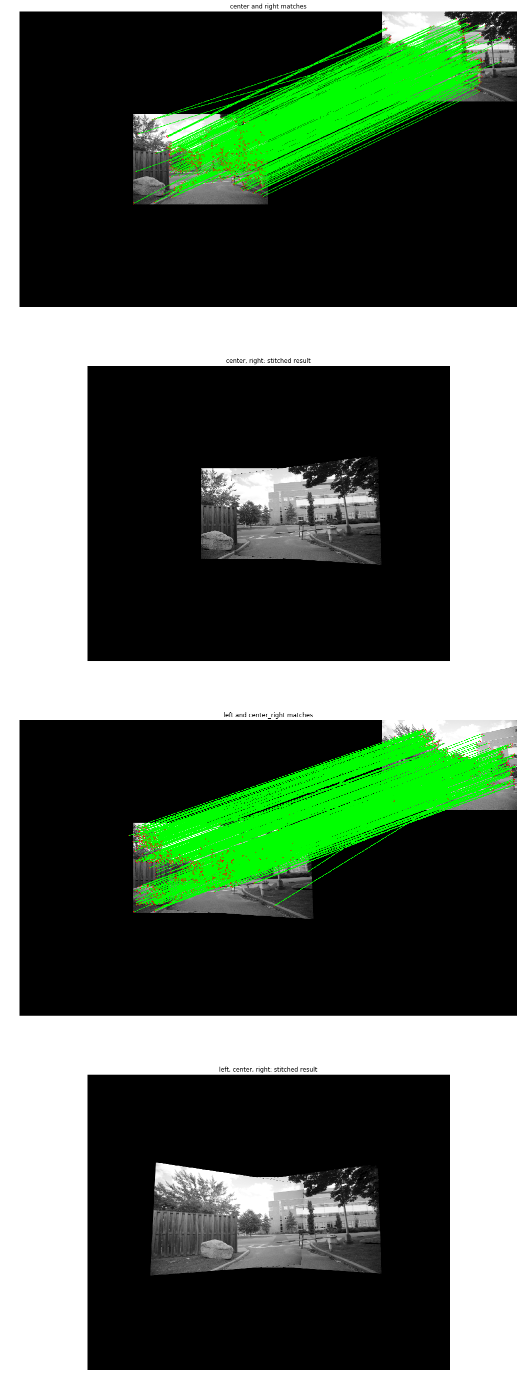
Step 1. Compute the transformation from the right image to the center image. Warp the right image with the computed transformation. Stitch the center and right images with alpha blending. Display the SIFT feature matching between the center and right images like you did in problem 1. Display the stitched result (center and right image).
Step 2 Compute the transformation from the left image to the stitched image from step 1. Warp the left image with the computed transformation. Stich the left and result images from step 1 with alpha blending. Display the SIFT feature matching between the result image from step 1 and the left image like what you did in problem 1. Display the final stitched result (all three images).
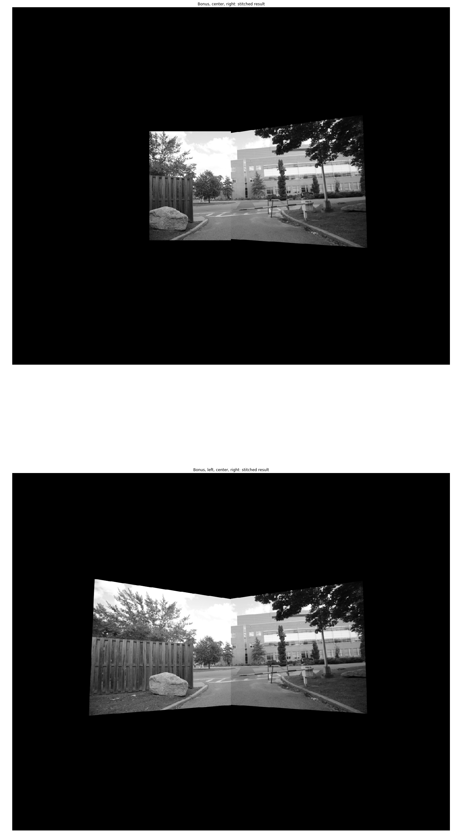
Bonus. Instead of using cv2.addWeighted to do the blending, implement Laplacian Pyramids to blend the two aligned images. Tutorials can be found at http://opencv-python-tutroals.readthedocs.io/en/latest/py_tutorials/py_imgproc/py_pyramids/py_pyramids.html. Display the stitched result (center and right image) and the final stitched result (all three images) with laplacian blending instead of alpha blending.

Note that for the resultant stitched image, some might have different intensity in the overlapping and other regions, namely the overlapping region looks brighter or darker than others. To get full credit, the final image should have uniform illumination.

Hints: You need to find the warping matrix between images with the same mechanism from problem 1. You will need as many reliable matches as possible to find a good homography so DO NOT use 0.1 here. A suggested value would be 0.75 in this case.

When you warp the image with cv2.warpPerspective, an important trick is to pass in the correct parameters so that the warped image has the same size with the padded_center image. Once you have two images with the same size, find the overlapping part and do the blending.

imgCenter = cv2.imread('SourceImages/stitch_m.jpg', 0)
imgRight  = cv2.imread('SourceImages/stitch_r.jpg', 0)
imgLeft   = cv2.imread('SourceImages/stitch_l.jpg', 0)

# initalize the stitched image as the center image
height, width = imgCenter.shape[:2]
imgCenter = cv2.copyMakeBorder(imgCenter, (1312 - height) / 2, (1312 - height) / 2, (1608 - width) / 2, (1608 - width) / 2, cv2.BORDER_CONSTANT)

# blend two images
def alpha_blend(img, warped):
    # Use image as ROI
    roi = img.copy()
    
    # Now create a mask of warped image and create its inverse mask
    ret, mask = cv2.threshold(warped, 10, 255, cv2.THRESH_BINARY)
    mask_inv = cv2.bitwise_not(mask)
    
    # Now black-out the area of warped image in ROI
    img_bg = cv2.bitwise_and(roi, roi, mask = mask_inv)
    
    # Take only region of warp from warped image.
    warped_fg = cv2.bitwise_and(warped, warped, mask = mask)
    
    # Put warped in ROI
    blended = cv2.add(img_bg, warped_fg)
    
    return blended

def Laplacian_Blending(A, B, mask, num_levels=1):
    # assume mask is float32 [0,1]

    # generate Gaussian pyramid for A,B and mask
    G = A.copy()
    gaussian_pyramid_A = [G]
    for i in xrange(num_levels):
        G = cv2.pyrDown(G)
        gaussian_pyramid_A.append(G)
        
    G = B.copy()
    gaussian_pyramid_B = [G]
    for i in xrange(num_levels):
        G = cv2.pyrDown(G)
        gaussian_pyramid_B.append(G)
    
    G = mask.copy()
    gaussian_pyramid_mask = [G]
    for i in xrange(num_levels):
        G = cv2.pyrDown(G)
        gaussian_pyramid_mask.append(G)
        
    # generate Laplacian Pyramids for A,B and masks
    laplacian_pyramid_A = [gaussian_pyramid_A[num_levels-1]]
    for i in xrange(num_levels-1, 0, -1):
        size = (gaussian_pyramid_A[i-1].shape[1], gaussian_pyramid_A[i-1].shape[0])
        GE = cv2.pyrUp(gaussian_pyramid_A[i], dstsize=size)
        L = cv2.subtract(gaussian_pyramid_A[i-1], GE)
        laplacian_pyramid_A.append(L)

    laplacian_pyramid_B = [gaussian_pyramid_B[num_levels-1]]
    for i in xrange(num_levels-1, 0, -1):
        size = (gaussian_pyramid_B[i-1].shape[1], gaussian_pyramid_B[i-1].shape[0])
        GE = cv2.pyrUp(gaussian_pyramid_B[i], dstsize=size)
        L = cv2.subtract(gaussian_pyramid_B[i-1], GE)
        laplacian_pyramid_B.append(L)

    laplacian_pyramid_mask = [gaussian_pyramid_mask[num_levels-1]]
    for i in xrange(num_levels-1, 0, -1):
        laplacian_pyramid_mask.append(gaussian_pyramid_mask[i-1])
        
    # Now blend images according to mask in each level
    blended_levels = []
    for level_a, level_b, level_m in zip(laplacian_pyramid_A, laplacian_pyramid_B, laplacian_pyramid_mask):
        blended_level = level_a * level_m + level_b * (1.0 - level_m)
        blended_levels.append(blended_level)

    # now reconstruct
    blended = blended_levels[0]
    for i in xrange(1, num_levels):
        size = (blended_levels[i].shape[1], blended_levels[i].shape[0])
        blended = cv2.pyrUp(blended, dstsize=size)
        blended = cv2.add(blended, blended_levels[i])

    return blended

def getTransform(img1, img2):
    # compute sift descriptors
    sift = cv2.xfeatures2d.SIFT_create()
    keypoints1, descriptors1 = sift.detectAndCompute(img1, None)
    keypoints2, descriptors2 = sift.detectAndCompute(img2, None)

    # find all mactches
    bf_matcher = cv2.BFMatcher()
    detected_matches = bf_matcher.knnMatch(descriptors1, descriptors2, k=2)
    
    # Apply ratio test
    good_matches = [] # Append filtered matches to this list
    for match in detected_matches:
        if match[0].distance < 0.75 * match[1].distance:
            good_matches.append(match[0])

    # draw matches
    img_match = drawMatches(img1, keypoints1, img2, keypoints2, good_matches)

    # estimate transform matrix using RANSAC
    source_points = np.float32([ keypoints1[m.queryIdx].pt for m in good_matches])
    destination_points = np.float32([ keypoints2[m.trainIdx].pt for m in good_matches])
    
    # find perspective transform matrix using RANSAC
    H, mask = cv2.findHomography(destination_points, source_points, cv2.RANSAC)
    
    return H, img_match

def perspective_warping(imgCenter, imgLeft, imgRight):
    
    # Get homography from right to center
    # ===== img_match1 is your first output =====
    T_R2C, img_match1 = getTransform(imgCenter, imgRight)
    
    # Blend center and right
    # ===== stitched_cr is your second output =====
    imgRightWarped = cv2.warpPerspective(imgRight, T_R2C , (imgCenter.shape[1], imgCenter.shape[0]))
    stitched_cr = alpha_blend(imgCenter, imgRightWarped)
    
    # Get homography from left to stitched center_right
    # ===== img_match2 is your third output =====
    T_L2CR, img_match2 = getTransform(stitched_cr, imgLeft)
    
    # Blend left and center_right
    # ===== stitched_res is your fourth output =====
    imgLeftWarped = cv2.warpPerspective(imgLeft, T_L2CR , (stitched_cr.shape[1], stitched_cr.shape[0]))
    stitched_res = alpha_blend(stitched_cr, imgLeftWarped)
    
    return stitched_res, stitched_cr, img_match1, img_match2

def perspective_warping_laplacian_blending(imgCenter, imgLeft, imgRight):
    
    # Get homography from right to center
    T_R2C, img_match1 = getTransform(imgCenter, imgRight)
    
    # Blend center and right
    # ===== This is your first bonus output =====
    imgRightWarped = cv2.warpPerspective(imgRight, T_R2C, (imgCenter.shape[1], imgCenter.shape[0]))
    mask = np.ones_like(imgCenter, dtype='float32')
    mask[:,int(mask.shape[1]/2):] = 0
    stitched_cr = Laplacian_Blending(imgCenter, imgRightWarped, mask, 1)
    
    # Get homography from left to stitched center_right
    T_L2CR, img_match2 = getTransform(stitched_cr.astype(np.uint8), imgLeft)
    
    # Blend left and center_right
    # ===== This is your second bonus output =====
    imgLeftWarped = cv2.warpPerspective(imgLeft, T_L2CR, (stitched_cr.shape[1], stitched_cr.shape[0]))
    mask = np.zeros_like(stitched_cr, dtype='float32')
    mask[:,mask.shape[1]/2:] = 1
    stitched_res = Laplacian_Blending(stitched_cr, imgLeftWarped, mask, 1)
    
    return stitched_res, stitched_cr


# ====== Plot functions, DO NOT CHANGE =====
stitched_res, stitched_cr, img_match1, img_match2 = perspective_warping(imgCenter, imgLeft, imgRight)
stitched_res_lap, stitched_cr_lap = perspective_warping_laplacian_blending(imgCenter, imgLeft, imgRight)
        
plt.figure(figsize=(25,50))
plt.subplot(4, 1, 1)
plt.imshow(img_match1, cmap='gray')
plt.title("center and right matches")
plt.axis('off')
plt.subplot(4, 1, 2)
plt.imshow(stitched_cr, cmap='gray')
plt.title("center, right: stitched result")
plt.axis('off')
plt.subplot(4, 1, 3)
plt.imshow(img_match2, cmap='gray')
plt.title("left and center_right matches")
plt.axis('off')
plt.subplot(4, 1, 4)
plt.imshow(stitched_res, cmap='gray')
plt.title("left, center, right: stitched result")
plt.axis('off')
plt.show()

plt.figure(figsize=(25,50))
plt.subplot(2, 1, 1)
plt.imshow(stitched_cr_lap, cmap='gray')
plt.title("Bonus, center, right: stitched result")
plt.axis('off')
plt.subplot(2, 1, 2)
plt.imshow(stitched_res_lap, cmap='gray')
plt.title("Bonus, left, center, right: stitched result")
plt.axis('off')
# =============================================

png

(-0.5, 1607.5, 1311.5, -0.5)

png

Problem 3: Object Recognition with HOG features

You will use the histogram of oriented gradients (HOG) to extract features from objects and recognize them.

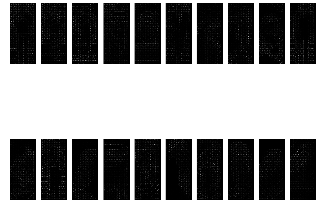
HOG decomposes an image into multiple cells, computes the direction of the gradients for all pixels in each cell, and creates a histogram of gradient orientation for that cell. Object recognition with HOG is usually done by extracting HOG features from a training set of images, learning a support vector machine (SVM) from those features, and then testing a new image with the SVM to determine the existence of an object.

You can use cv2.HOGDescriptor to extract the HoG feature and cv2.ml.SVM_create for SVMs (and a lot of other algorithms). You can also use Python machine learning packages for SVM, e.g.scikit-learn and for HoG computation, e.g. scikit-image. Please find the OpenCV SVM tutorial at https://www.learnopencv.com/handwritten-digits-classification-an-opencv-c-python-tutorial/.

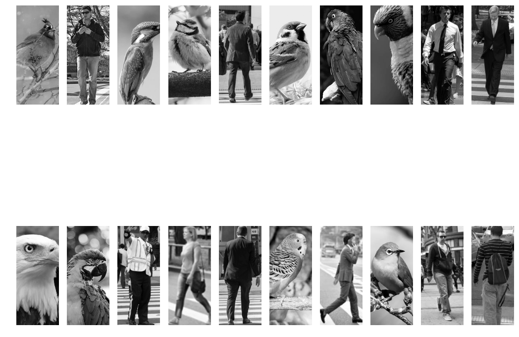
An image set located under SourceImages/human_vs_birds is provided containing 20 images. You will first train an SVM with the HoG features and then predict the class of an image with the trained SVM. For simplicity, we will be dealing with a binary classification problem with two classes, namely, birds and humans. There are 10 images for each class.

Some of the function names and arguments are provided, you may change them as you see fit.

Step 1. Load in the images and create a vector of corresponding labels (0 for bird and 1 for human). An example label vector should be something like [1,1,1,1,1,0,0,0,0,0]. Shuffle the images randomly and display them in a 2 x 10 grid with figsize = (18, 15).
Step 2. Extract HoG features from all images. You can use the OpenCV function cv2.HOGDescriptor or hog routine from scikit-image. Display the HoG features for all images in a 2 x 10 grid with figsize = (18, 15).
Step 3. Use the first 16 examples from the shuffled dataset as training data on which to train an SVM. The rest 4 are used as test data. Reshape the HoG feature matrix as necessary to feed into the SVM. Train the classifier. DO NOT train with test data. No output is expected from this part.
Step 4. Perform predictions with your trained SVM on the test data. Output a vector of predictions, a vector of ground truth labels, and prediction accuracy.

# load data
def loadData(filepath, file_start):
  files = [ f for f in listdir(filepath) if isfile(join(filepath, f)) and f.startswith(file_start) ]
  images = np.empty(len(files), dtype=object)
  for n in range(0, len(files)):
    images[n] = cv2.imread(join(filepath, files[n]), 0)
    
  return images
    
# create a vector of labels
# assume labels: bird = 0, human = 1
bird_images = loadData('SourceImages/human_vs_birds/', 'bird_')
label_vector = [0 for image in bird_images]
human_images = loadData('SourceImages/human_vs_birds/', 'human_')
label_vector.extend([1 for image in human_images])

images = []
images.extend(bird_images)
images.extend(human_images)

# Random shuffle of images and corresponding label vector
rng_state = np.random.get_state()
np.random.shuffle(images)
np.random.set_state(rng_state)
np.random.shuffle(label_vector)

# ===== Display your first graph here =====
plt.figure(figsize=(18,15))
rows = 2
cols = 10
for i in range(1, len(images)+1):
  plt.subplot(rows, cols, i)
  plt.imshow(images[i-1], cmap='gray')
  plt.axis('off')

plt.show()

png

# Compute HOG features for the images
def computeHOGfeatures(image):
    feature_descriptor, hog_image = hog(image, orientations=8, pixels_per_cell=(16, 16), cells_per_block=(1, 1), visualize=True)

    return feature_descriptor, hog_image


# Compute HOG descriptors
hog_features = []
hog_images = []
for image in images:
  feature_descriptor, hog_image = computeHOGfeatures(image)
  hog_features.append(feature_descriptor)
  hog_images.append(hog_image)
  

# ===== Display your second graph here =====
plt.figure(figsize=(18,15))
rows = 2
cols = 10
for i in range(1, len(hog_images)+1):
  plt.subplot(rows, cols, i)
  plt.imshow(hog_images[i-1], cmap='gray')
  plt.axis('off')

plt.show()
  
# reshape feature matrix
hog_features = np.array(hog_features)
labels = np.array(label_vector).reshape(len(label_vector), 1)
data_frame = np.hstack((hog_features, labels))
print data_frame.shape

# Split the data and labels into train and test set
x_train, x_test = hog_features[:16], hog_features[16:]
y_train, y_test = labels[:16] , labels[16:]
print x_train.shape, x_test.shape
print y_train.shape, y_test.shape

png

(20, 2001)
(16, 2000) (4, 2000)
(16, 1) (4, 1)

# train model with SVM
# call LinearSVC
classifier = svm.LinearSVC()
# train SVM
classifier.fit(x_train, y_train)
# call clf.predict
y_pred = classifier.predict(x_test)

# ===== Output functions ======
print 'estimated labels: ', y_pred
print 'ground truth labels: ', y_test
print 'Accuracy: ', str(accuracy_score(y_test, y_pred) * 100), '%'

estimated labels:  [1 0 0 0]
ground truth labels:  [[1]
 [0]
 [0]
 [0]]
Accuracy:  100.0 %

Narayan Acharya

Computer Vision Assignment 2

NOTE: Using SIFT in OpenCV 3.x.x

Some Resources

Problem 1: Match transformed images using SIFT features

Problem 2: Scene stitching with SIFT features

Problem 3: Object Recognition with HOG features

You may also enjoy

Answering Questions About Stony Brook

Summer 2020 At Playstation!

Sem2 Update

New Macbook Pro 16!