Computer Vision Assignment 1

This is the first of the 6 assignments I did as part of the Computer Vision course (CSE-527) during Fall 19 at Stony Brook University. The assignment covers the following topics:

1. Gaussian Convolution
2. Median Filtering
3. Separable Convolutions
4. Laplacian of Gaussian
5. Histogram Equalization
6. Low Pass and High Pass Filters

This assignment requires familiarity with Python (v3.x). Other Python packages required are numpy, matplotlib and opencv-python. I used Google Colab for the purposes of this assignment, though one can complete the same using a local setup of Jupyter. I don’t dive into the details of getting up and running with python or jupyter as there are a lot of other resources one can use to get started with these topics.

IMPORTANT NOTE: The images used in this assignment can be found here

Install Python packages: install Python packages: numpy, matplotlib, opencv-python using pip, for example:

pip install numpy matplotlib opencv-python

Next we import the modules that we might need during the course of this assignment.

import math
import sys
import cv2
import numpy as np
import matplotlib.pyplot as plt
from scipy import ndimage, misc
from IPython.display import display, Image
from mpl_toolkits.mplot3d import Axes3D
from matplotlib import cm

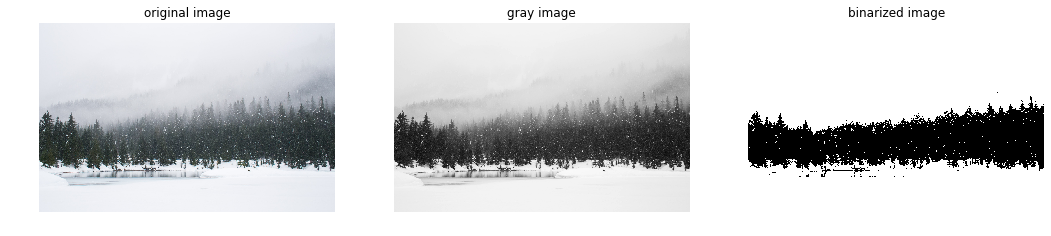
Below is a simple example for image thresholding. This was just an introductory piece and was not graded as part of the assignment.

# function for image thresholding
def imThreshold(img, threshold, maxVal):
    assert len(img.shape) == 2 # input image has to be gray
    
    height, width = img.shape
    bi_img = np.zeros((height, width), dtype=np.uint8)
    for x in range(height):
        for y in range(width):
            if img.item(x, y) > threshold:
                bi_img.itemset((x, y), maxVal)
                
    return bi_img

# read the image for local directory (same with this .ipynb) 
img = cv2.imread('SourceImages/Snow.jpg')

# convert a color image to gray
img_gray = cv2.cvtColor(img, cv2.COLOR_BGR2GRAY)

# image thresholding using global tresholder
img_bi = imThreshold(img_gray, 127, 255)

# Be sure to convert the color space of the image from
# BGR (Opencv) to RGB (Matplotlib) before you show a 
# color image read from OpenCV
plt.figure(figsize=(18, 6))
plt.subplot(1, 3, 1)
plt.imshow(cv2.cvtColor(img, cv2.COLOR_BGR2RGB))
plt.title('original image')
plt.axis("off")

plt.subplot(1, 3, 2)
plt.imshow(img_gray, 'gray')
plt.title('gray image')
plt.axis("off")

plt.subplot(1, 3, 3)
plt.imshow(img_bi, 'gray')
plt.title('binarized image')
plt.axis("off")

plt.show()

Problems

---

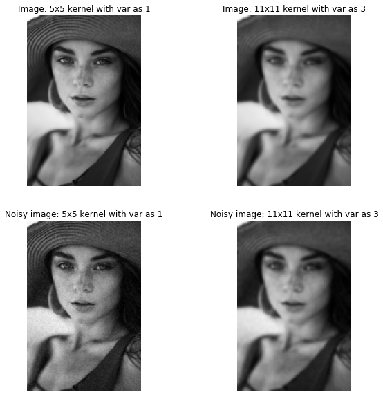
• Problem 1.a Gaussian convolution:
  Write a function in Python that takes two arguments, a width parameter and a variance parameter, and returns a 2D array containing a Gaussian kernel of the desired dimension and variance. The peak of the Gaussian should be in the center of the array. Make sure to normalize the kernel such that the sum of all the elements in the array is 1. Use this function and the OpenCV’s filter2D routine to convolve the image and noisy image arrays with a 5 by 5 Gaussian kernel with sigma of 1. Repeat with a 11 by 11 Gaussian kernel with a sigma of 3. There will be four output images from this problem, namely, image convolved with 3x3, 11x11, noisy image convolved with 3x3, and 11x11. Once you fill in and run the codes, the outputs will be saved under Results folder.

def genGaussianKernel(width, sigma):
    # define your 2d kernel here
    kernel_2d = np.zeros((width, width))
    
    # Prepare variables for computation
    center = int(width / 2)
    sigma_squared = sigma * sigma
    coeff = 1 / (2 * math.pi * sigma_squared)
    
    for i in range(width):
      for j in range(width):
        power = -((i - center)**2 + (j - center)**2) / (2 * sigma_squared)
        kernel_2d[i,j] = coeff * (math.e ** power) 
    
    # Return a normalized matrix, sum of all numbers adds up to 1
    return kernel_2d / kernel_2d.sum()

# Load images
img       = cv2.imread('SourceImages/pic.jpg', 0)
img_noise = cv2.imread('SourceImages/pic_noisy.jpg', 0)

# Generate Gaussian kernels
kernel_1 = genGaussianKernel(5, 1)      # 5 by 5 kernel with sigma of 1
kernel_2 = genGaussianKernel(11, 3)      # 11 by 11 kernel with sigma of 3

# Take a look at generated Gaussian kernels
# plt.imshow(kernel_1)
# plt.imshow(kernel_2)

# Convolve with image and noisy image
res_img_kernel1 = cv2.filter2D(img, -1, kernel_1)
res_img_kernel2 = cv2.filter2D(img, -1, kernel_2)
res_img_noise_kernel1 = cv2.filter2D(img_noise, -1, kernel_1)
res_img_noise_kernel2 = cv2.filter2D(img_noise, -1, kernel_2)

# Write out result images
cv2.imwrite("Results/P1_01.jpg", res_img_kernel1)
cv2.imwrite("Results/P1_02.jpg", res_img_kernel2)
cv2.imwrite("Results/P1_03.jpg", res_img_noise_kernel1)
cv2.imwrite("Results/P1_04.jpg", res_img_noise_kernel2)

# Plot results
plt.figure(figsize = (10, 10))
plt.subplot(2, 2, 1)
plt.imshow(res_img_kernel1, 'gray')
plt.title('Image: 5x5 kernel with var as 1')
plt.axis("off")

plt.subplot(2, 2, 2)
plt.imshow(res_img_kernel2, 'gray')
plt.title('Image: 11x11 kernel with var as 3')
plt.axis("off")

plt.subplot(2, 2, 3)
plt.imshow(res_img_noise_kernel1, 'gray')
plt.title('Noisy image: 5x5 kernel with var as 1')
plt.axis("off")

plt.subplot(2, 2, 4)
plt.imshow(res_img_noise_kernel2, 'gray')
plt.title('Noisy image: 11x11 kernel with var as 3')
plt.axis("off")

plt.show()

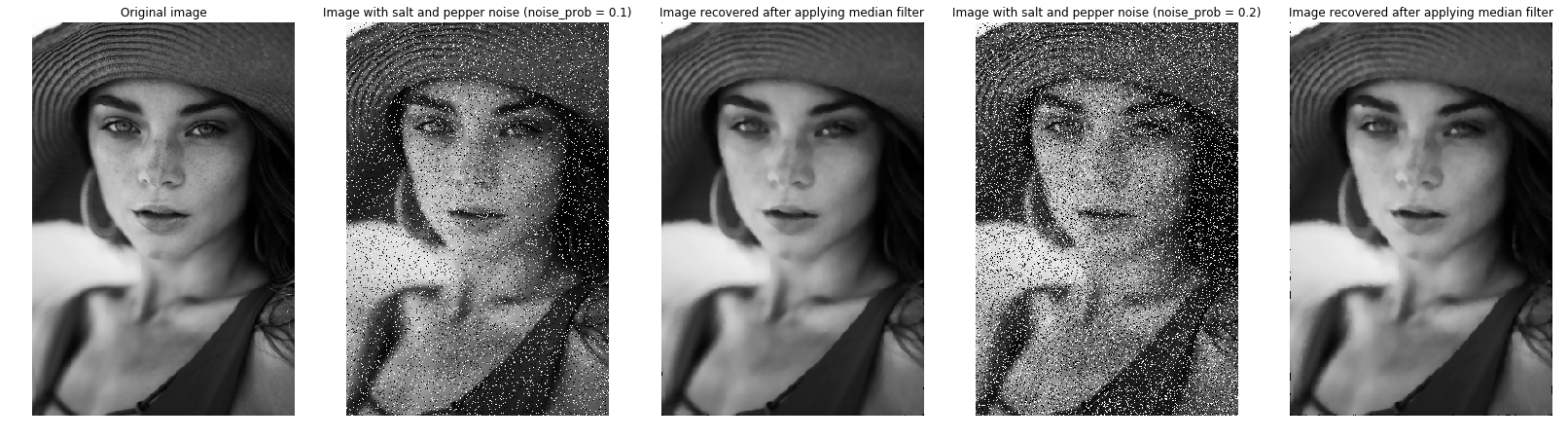
• Problem 1.b Median filter:
  (a)Write a function to generate an image with salt and pepper noise. The function takes two arguments, the input image and the probability that a pixel location has salt-pepper noise. A simple implementation can be to select pixel locations with probability ‘p’ where noise occurs and then with equal probability set the pixel value at those location to be 0 or 255.(Hint: Use np.random.uniform())
  (b)Write a function to implement a median filter. The function takes two arguments, an image and a window size(if window size is ‘k’, then a kxk window is used to determine the median pixel value at a location) and returns the output image. Do not use any inbuilt library (like scipy.ndimage_filter) to directly generate the result.
  For this question display the outputs for “probabilty of salt and pepper noise” argument in the noisy_image_generator function equal to 0.1 and 0.2, and median filter window size in median_filter function equal to 5x5.
  (c) What is the Gaussian filter size (and sigma) that achieves a similar level of noise removal.

# Function to generate image with salt and pepper noise
def noisy_image_generator(img_in, probability = 0.1):
  # define your function here
  # Fill in your code here
  height, width = img_in.shape
  img_out = np.zeros((height, width))
  
  # Generate a uniform distribution array of input image shape
  # Numbers lie between 0 and 1 and are equally distributed
  noise = np.random.uniform(0, 1, (height, width))
  for i in range(height):
    for j in range(width):
      # Check if this pixel can be picked for choice of noisy pixel
      if noise[i][j] < probability:
        # Helps generate 0 or 1 with equal probability
        black_or_white = np.random.choice(2, 1)
        img_out[i][j] = 255 if black_or_white[0] == 1 else 0
      else:
        img_out[i][j] = img_in[i][j]
  
  return img_out
  
# Function to apply median filter(window size kxk) on the input image  
def median_filter(img_in, window_size = 5):
  # define your function here
  # Fill in your code here
  
  k = int(window_size / 2)
  
  # Add k black pixel padding to the top, bottom, left and right 
  # so median filter window can run over all pixels of original image
  img_in_with_border = cv2.copyMakeBorder(img_in, k , k, k, k,
                                          cv2.BORDER_CONSTANT, value=(0, 0, 0))
  height, width = img_in_with_border.shape
  img_out = img_in_with_border.copy()
  
  for i in range(k, height-k):
    for j in range(k, width-k):
      window = img_in_with_border[i-k:i+k+1, j-k:j+k+1]
      median = np.median(window)
      img_out[i][j] = median
        
  # Crop out the k pixel padding added before returning output image
  return img_out[k:height-k, k:width-k]
  
image_s_p1 = noisy_image_generator(img, probability = 0.1)  
result1 = median_filter(image_s_p1, window_size = 5)

image_s_p2 = noisy_image_generator(img, probability = 0.2)  
result2 = median_filter(image_s_p2, window_size = 5)

cv2.imwrite("Results/P1_05.jpg", result1)    
cv2.imwrite("Results/P1_06.jpg", result2)

# Plot results
plt.figure(figsize = (28, 20))
plt.subplot(1, 5, 1)
plt.imshow(img, 'gray')
plt.title('Original image')
plt.axis("off")

plt.subplot(1, 5, 2)
plt.imshow(image_s_p1, 'gray')
plt.title('Image with salt and pepper noise (noise_prob = 0.1)')
plt.axis("off")

plt.subplot(1, 5, 3)
plt.imshow(result1, 'gray')
plt.title('Image recovered after applying median filter')
plt.axis("off")

plt.subplot(1, 5, 4)
plt.imshow(image_s_p2, 'gray')
plt.title('Image with salt and pepper noise (noise_prob = 0.2)')
plt.axis("off")

plt.subplot(1, 5, 5)
plt.imshow(result2, 'gray')
plt.title('Image recovered after applying median filter')
plt.axis("off")

plt.show()

print("Gaussian Filter Results")

# TODO: Tweak with GF below to mimic Median Filter results
gf = genGaussianKernel(15, 5)

# Running above GF on noisy image with 0.1 probability
result3 = cv2.filter2D(image_s_p1, -1, gf)

# Running above GF on noisy image with 0.2 probability
result4 = cv2.filter2D(image_s_p2, -1, gf)

# Plot results
plt.figure(figsize = (28, 20))

plt.subplot(2, 5, 1)
plt.imshow(img, 'gray')
plt.title('Original image')
plt.axis("off")

plt.subplot(2, 5, 2)
plt.imshow(image_s_p1, 'gray')
plt.title('Image with salt and pepper noise (noise_prob = 0.1)')
plt.axis("off")

plt.subplot(2, 5, 3)
plt.imshow(result3, 'gray')
plt.title('Image recovered after applying GF(5x5, sigma=1)')
plt.axis("off")

plt.subplot(2, 5, 4)
plt.imshow(image_s_p2, 'gray')
plt.title('Image with salt and pepper noise (noise_prob = 0.2)')
plt.axis("off")

plt.subplot(2, 5, 5)
plt.imshow(result4, 'gray')
plt.title('Image recovered after applying GF(5x5, sigma=1)')
plt.axis("off")

plt.show()

Gaussian Filter Results

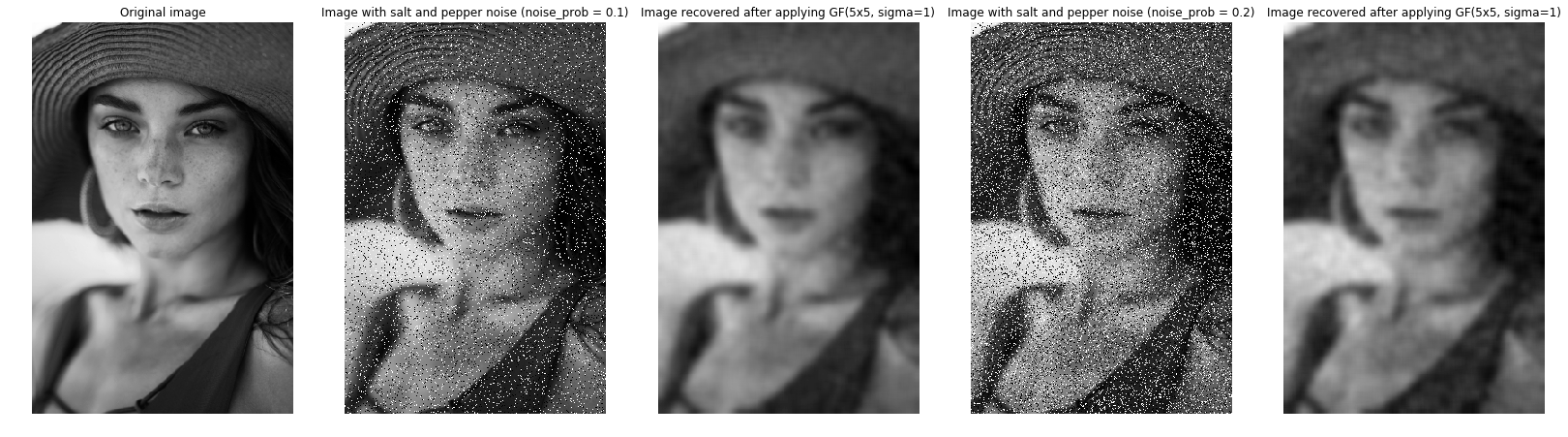
Note for 1.b.c:

Even though Gaussian Filter was able to remove most, if not all, noise it performs poorly compared to Median Filter with respect to Salt and Pepper Noise. Gaussuan Filter ends up losing essential features because of blurring with larger window and higher sigma to remove noisy pixels.

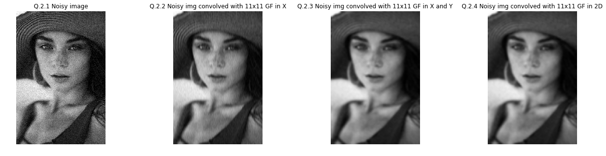
• Problem 2 Separable convolutions:
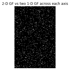
  The Gaussian kernel is separable, which means that convolution with a 2D Gaussian can be accomplished by convolving the image with two 1D Gaussians, one in the x direction and the other one in the y direction. Perform an 11x11 convolution with sigma = 3 from question 1 using this scheme. You can still use filter2D to convolve the images with each of the 1D kernels. Verify that you get the same results with what you did with 2D kernels by computing the difference image between the results from the two methods.

def genGausKernel1D(length, sigma):
    
    # define you 1d kernel here
    kernel_1d = np.zeros((length, 1))
    
    # Prepare variables for computation
    center = int(length / 2)
    sigma_squared = sigma * sigma
    coeff = 1 / math.sqrt(2 * math.pi * sigma_squared)
    
    for i in range(length):
      power = -((i - center)**2) / (2 * sigma_squared)
      kernel_1d[i] = coeff * (math.e ** power) 
    
    # Return a normalized array, sum of all numbers adds up to 1
    return kernel_1d / kernel_1d.sum()

# Generate two 1d kernels here
width = 11
sigma = 3
kernel_x = genGausKernel1D(width, sigma)
kernel_y = np.transpose(kernel_x)

# print(kernel_x, "\n", kernel_y)

# Generate a 2d 11x11 kernel with sigma of 3 here as before
kernel_2d = genGaussianKernel(width, sigma) 

# Convolve with img_noise
res_img_noise_kernel1d_x  = cv2.filter2D(img_noise, -1, kernel_x)
res_img_noise_kernel1d_xy = cv2.filter2D(res_img_noise_kernel1d_x, -1, kernel_y)
res_img_noise_kernel2d    = cv2.filter2D(img_noise, -1, kernel_2d)

# Plot results
plt.figure(figsize=(22, 5))
plt.subplot(1, 4, 1)
plt.imshow(img_noise, 'gray')
plt.title('Q.2.1 Noisy image')
plt.axis("off")

plt.subplot(1, 4, 2)
plt.imshow(res_img_noise_kernel1d_x, 'gray')
plt.title('Q.2.2 Noisy img convolved with 11x11 GF in X')
plt.axis("off")

plt.subplot(1, 4, 3)
plt.imshow(res_img_noise_kernel1d_xy, 'gray')
plt.title('Q.2.3 Noisy img convolved with 11x11 GF in X and Y')
plt.axis("off")

plt.subplot(1, 4, 4)
plt.imshow(res_img_noise_kernel2d, 'gray')
plt.title('Q.2.4 Noisy img convolved with 11x11 GF in 2D')
plt.axis("off")

plt.show()

# Compute the difference array here
img_diff = cv2.subtract(res_img_noise_kernel2d, res_img_noise_kernel1d_xy)
plt.imshow(img_diff, 'gray')
plt.title('2-D GF vs two 1-D GF across each axis')
plt.axis("off")

plt.show()

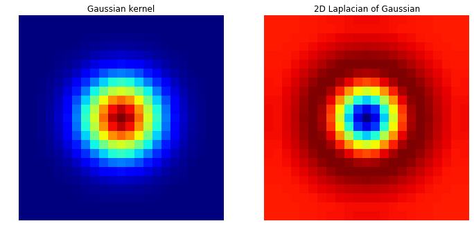
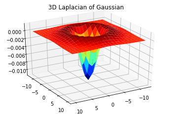
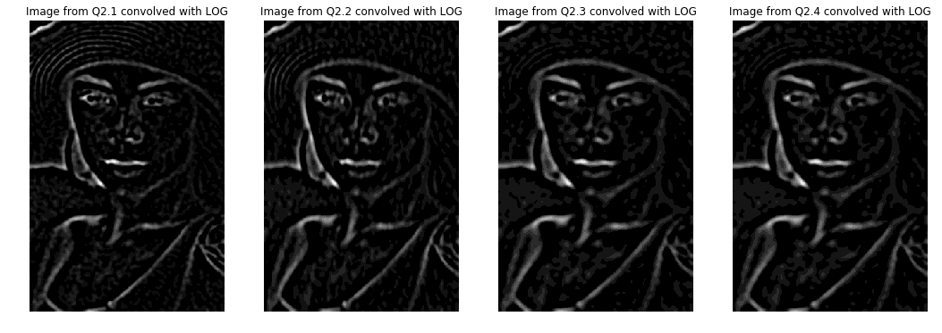
• Problem 3 Laplacian of Gaussian:
  Convolve a 23 by 23 Gaussian of sigma = 3 with the discrete approximation to the Laplacian kernel [1 1 1; 1 -8 1; 1 1 1]. Plot the Gaussian kernel and 2D Laplacian of Gaussian using the Matplotlib function plot. Use the Matplotlib function plot_surface to generate a 3D plot of LoG. Do you see why this is referred to as the Mexican hat filter? Include your code and results in your Colab Notebook file. Apply the filter to the four output images generated in the previous question.

width = 23
sigma = 3

# Create your Laplacian kernel
Laplacian_kernel = np.array([[1, 1, 1], [1, -8, 1], [1, 1, 1]])

# Create your Gaussian kernel
Gaussian_kernel = genGaussianKernel(width, sigma)

# Create your Laplacian of Gaussian
LoG = cv2.filter2D(Gaussian_kernel, -1, Laplacian_kernel)

# Plot Gaussian and Laplacian
fig = plt.figure(figsize=(18, 6))
plt.subplot(1, 3, 1)
plt.imshow(Gaussian_kernel, interpolation='none', cmap=cm.jet)
plt.title('Gaussian kernel')
plt.axis("off")

plt.subplot(1, 3, 2)
plt.imshow(LoG, interpolation='none', cmap=cm.jet)
plt.title('2D Laplacian of Gaussian')
plt.axis("off")

# Plot the 3D figure of LoG
# Fill in your code here
fig_3d = plt.figure()
ax = fig_3d.gca(projection='3d')
ax.view_init(30, 60)
X = [i for i in range(-len(LoG) // 2, len(LoG) // 2)]
Y = [i for i in range(-len(LoG[0]) // 2, len(LoG[0]) // 2)]
X, Y = np.meshgrid(X, Y)
surf = ax.plot_surface(X, Y, LoG, cmap=cm.jet)
plt.title('3D Laplacian of Gaussian')

img_noise_LOG = cv2.filter2D(img_noise, -1, LoG)
res_img_noise_kernel1d_x_LOG =  cv2.filter2D(res_img_noise_kernel1d_x, -1, LoG)
res_img_noise_kernel1d_xy_LOG = cv2.filter2D(res_img_noise_kernel1d_xy, -1, LoG)
res_img_noise_kernel2d_LOG = cv2.filter2D(res_img_noise_kernel2d, -1, LoG)


# Plot results
plt.figure(figsize=(18, 6))
plt.subplot(1, 4, 1)
plt.imshow(img_noise_LOG, 'gray')
plt.title('Image from Q2.1 convolved with LOG')
plt.axis("off")

plt.subplot(1, 4, 2)
plt.imshow(res_img_noise_kernel1d_x_LOG, 'gray')
plt.title('Image from Q2.2 convolved with LOG')
plt.axis("off")

plt.subplot(1, 4, 3)
plt.imshow(res_img_noise_kernel1d_xy_LOG, 'gray')
plt.title('Image from Q2.3 convolved with LOG')
plt.axis("off")

plt.subplot(1, 4, 4)
plt.imshow(res_img_noise_kernel2d_LOG, 'gray')
plt.title('Image from Q2.4 convolved with LOG')
plt.axis("off")

plt.show()

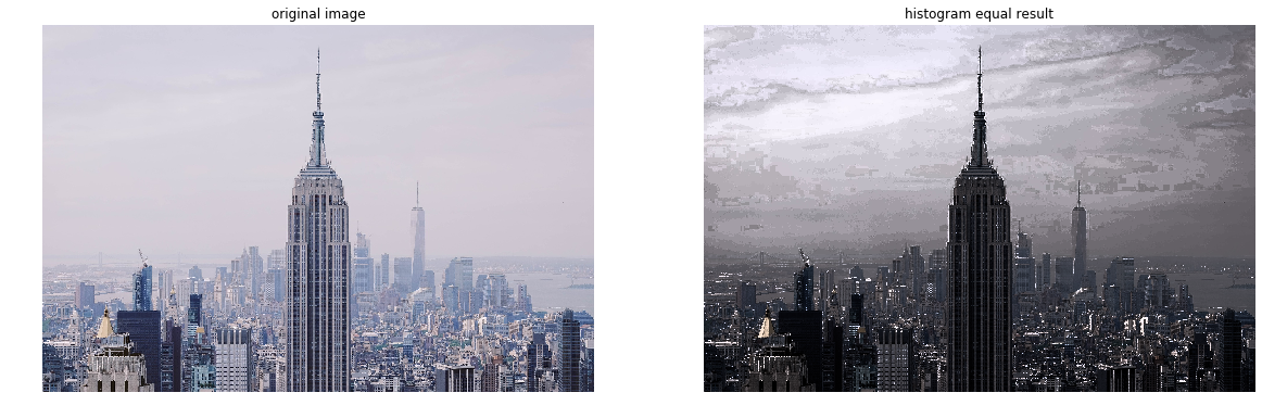
• Problem 4 Histogram equalization:
  Refer to Szeliski’s book on section 3.4.1, and within that section to eqn 3.9 for more information on histogram equalization. Getting the histogram of a grayscale image is incredibly easy with python. A histogram is a vector of numbers. Once you have the histogram, you can get the cumulative distribution function (CDF) from it. Then all you have left is to find the mapping from each value [0,255] to its adjusted value (just using the CDF basically). DO NOT use cv2.equalizeHist() directly to solve the exercise!

def histogram_equalization(img_in):

    # Write histogram equalization here
    # Fill in your code here
    
    # Figure for plotting histograms and graphs
#     fig = plt.figure(figsize=(20, 5))
    
    # Changing color space of image to HSV
    # We will only be equalizing the Value(V) space of the image
    # that corresponds with the brightness of the pixels
    hsv_image = cv2.cvtColor(img_in, cv2.COLOR_BGR2HSV)
    hue, saturation, value = cv2.split(hsv_image)
    
    # Using 256 Bins as V ranges from 0-255
    bins = 256
    
    # Flatten image into 1d array
    flat_img_in = value.flatten()
    # Plot Histogram to see skew in pixel V values
#     plt.subplot(1, 3, 1)
#     plt.title('V values Histogram')
#     plt.hist(flat_img_in, bins)
    
    # Iterate over the pixels to populate histogram buckets for V
    histogram = np.zeros(bins)
    for pixel in flat_img_in:
        histogram[pixel] += 1
    
    # Calculate CDF of Histogram
    a = iter(histogram)
    b = [next(a)]
    for i in a:
        b.append(b[-1] + i)
    cumulative_sums = np.array(b)
    # Plot above CDF
#     plt.subplot(1, 3, 2)
#     plt.title('CDF of Histogram')
#     plt.plot(cumulative_sums)
    
    # Re-normalize cumulative sum values to be between 0-255
    M = (cumulative_sums - cumulative_sums.min()) * (bins - 1)
    N = cumulative_sums.max() - cumulative_sums.min()
    cumulative_sums = M / N
  
    # Cast it back to uint8 (Floats now allowed in images)
    cumulative_sums = cumulative_sums.astype('uint8')
    
    # Get value from cumulative sum for all in flattened image of V
    equalized_v_values = cumulative_sums[flat_img_in]
#     plt.subplot(1, 3, 3)
#     plt.title('V values Equalized Histogram')
#     plt.hist(equalized_v_values, bins)
    
    # Put V back into original shape
    new_v_values = np.reshape(equalized_v_values, value.shape)
    img_out_hsv = cv2.merge([hue, saturation, new_v_values])
    
    # Go back to RGB color space
    img_out = cv2.cvtColor(img_out_hsv, cv2.COLOR_HSV2BGR)
    
    return True, img_out

# Read in input images
img_equal = cv2.imread('SourceImages/hist_equal.jpg', cv2.IMREAD_COLOR)

# Histogram equalization
succeed, output_image = histogram_equalization(img_equal)

# Plot results
fig = plt.figure(figsize=(20, 15))
plt.subplot(1, 2, 1)
plt.imshow(img_equal[..., ::-1])
plt.title('original image')
plt.axis("off")

# Plot results
plt.subplot(1, 2, 2)
plt.imshow(output_image[..., ::-1])
plt.title('histogram equal result')
plt.axis("off")

# Write out results
cv2.imwrite("Results/P4_01.jpg", output_image)

True

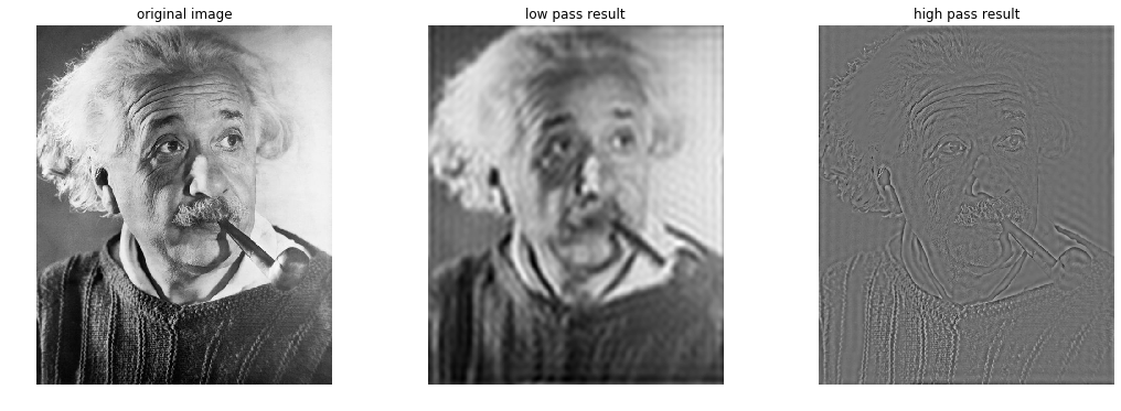
• Problem 5 Low and high pass filters: Start with the following tutorials:
  http://docs.opencv.org/master/de/dbc/tutorial_py_fourier_transform.html http://docs.opencv.org/2.4/doc/tutorials/core/discrete_fourier_transform/discrete_fourier_transform.html
  For your LPF (low pass filter), mask a 60x60 window of the center of the FT (Fourier Transform) image (the low frequencies). For the HPF, mask a 20x20 window excluding the center.

def low_pass_filter(img_in):

    # Write low pass filter here
    # Fill in your code here
    f = np.fft.fft2(img_in)
    fshift = np.fft.fftshift(f)
    
    # Only to plot frequency mag spectrum of image, not used as such
    magnitude_spectrum = 20 * np.log(np.abs(fshift))
    
    # mask
    # Fill in your code here
    rows, cols = img_in.shape
    crow, ccol = rows//2 , cols//2
    for i in range(rows):
      for j in range(cols):
        if (i >= crow - 30 and i < crow + 31) and (j >= ccol - 30 and j < ccol + 31):
          continue
        else:
          fshift[i, j] = 0
    
#     plt.subplot(131),plt.imshow(img_in, cmap = 'gray')
#     plt.title('Input Image'), plt.xticks([]), plt.yticks([])
#     plt.subplot(132),plt.imshow(magnitude_spectrum, cmap = 'gray')
#     plt.title('Magnitude Spectrum'), plt.xticks([]), plt.yticks([])
#     plt.subplot(133),plt.imshow(np.array(fshift, dtype=np.uint8), cmap = 'gray')
#     plt.title('Mask'), plt.xticks([]), plt.yticks([])
#     plt.show()
    
    # apply mask and inverse DFT
    # Fill in your code here
    f_ishift = np.fft.ifftshift(fshift)
    img_back = np.fft.ifft2(f_ishift)
    img_back = np.real(img_back)

    return True, img_back


def high_pass_filter(img_in):

    # Write high pass filter here
    # Fill in your code here
    f = np.fft.fft2(img_in)
    fshift = np.fft.fftshift(f)

    # Only to plot frequency mag spectrum of image, not used as such
    magnitude_spectrum = 20 * np.log(np.abs(fshift))
    
    # mask
    # Fill in your code here
    rows, cols = img_in.shape
    crow, ccol = rows//2 , cols//2
    fshift[crow-30:crow+31, ccol-30:ccol+31] = 0
    
#     plt.subplot(131),plt.imshow(img_in, cmap = 'gray')
#     plt.title('Input Image'), plt.xticks([]), plt.yticks([])
#     plt.subplot(132),plt.imshow(magnitude_spectrum, cmap = 'gray')
#     plt.title('Magnitude Spectrum'), plt.xticks([]), plt.yticks([])
#     plt.subplot(133),plt.imshow(np.array(fshift, dtype=np.uint8), cmap = 'gray')
#     plt.title('Mask'), plt.xticks([]), plt.yticks([])
#     plt.show()
    
    # apply mask and inverse DFT
    # Fill in your code here
    f_ishift = np.fft.ifftshift(fshift)
    img_back = np.fft.ifft2(f_ishift)
    img_back = np.real(img_back)
    
    return True, img_back

# Read in input images
img_filter = cv2.imread('SourceImages/Einstein.jpg', 0)

# Low and high pass filter
succeed1, output_low_pass_image1  = low_pass_filter(img_filter)
succeed2, output_high_pass_image2 = high_pass_filter(img_filter)

# Plot results
fig = plt.figure(figsize=(18, 6))
plt.subplot(1, 3, 1)
plt.imshow(img_filter, 'gray')
plt.title('original image')
plt.axis("off")

plt.subplot(1, 3, 2)
plt.imshow(output_low_pass_image1, 'gray')
plt.title('low pass result')
plt.axis("off")

plt.subplot(1, 3, 3)
plt.imshow(output_high_pass_image2, 'gray')
plt.title('high pass result')
plt.axis("off")

# Write out results
cv2.imwrite("Results/P5_01.jpg", output_low_pass_image1)
cv2.imwrite("Results/P5_02.jpg", output_high_pass_image2)

True

This wraps up the first of the 6 assignments I completed as part of the Computer Vision course during Fall 19. The assignment was pretty basic and helped with gaining familiarity with OpenCV for Python as well as help solidify concepts like Gaussian and Median Filtering, Separable Filters, Histogram Equalization and High Pass/Low Pass Filters that we saw in class.

Peace!