
Scene Recognition Using Convolutional Neural Networks
This is the fourth assignment for the Computer Vision (CSE-527) course from Fall 19 at Stony Brook University. As part of this assignment I learnt introductory Deep Learning techniques and its applications in Computer Vision related tasks. As part of this assignment, we design and train a Deep Convolutional Neural Network for scene recognition using PyTorch.
Remember Homework 3: Scene recognition with bag of words where we used a bag of features representation for 16-way scene classification. We’re going to attack the same task with deep learning and get higher accuracy. Training from scratch won’t work quite as well as homework 3 due to the insufficient amount of data, fine-tuning an existing network will work much better than homework 3.
In Problem 1 of the project we train a deep convolutional network from scratch to recognize scenes. We define a simple network architecture and add jittering, normalization, and regularization to increase recognition accuracy. Unfortunately, we only have 2,400 training examples so it doesn’t seem possible to train a network from scratch which outperforms hand-crafted features.
For Problem 2 we fine-tune a pre-trained deep network to achieve about 85% accuracy on the task. We will use the pretrained AlexNet network which was not trained to recognize scenes at all.
These two approaches represent the most common approaches to recognition problems in computer vision today – train a deep network from scratch if you have enough data (it’s not always obvious whether or not you do), and if you cannot then instead fine-tune a pre-trained network.
Dataset
Save the dataset(click me) into your working folder in your Google Drive for this homework. Under your root folder, there should be a folder named “data” containing the images.
Some Tutorials (PyTorch)
- PyTorch for deep learning toolbox (follow the link for installation).
- For PyTorch beginners, please read this tutorial before doing your homework.
- Feel free to study more tutorials at http://pytorch.org/tutorials/.
- Find cool visualization here at http://playground.tensorflow.org.
Gettin Started
# import packages here
import cv2
import numpy as np
import matplotlib.pyplot as plt
import glob
import random
import time
import os

import torch
import torchvision
from torchvision import datasets, models, transforms

from torch.autograd import Variable
import torch.nn as nn
import torch.nn.functional as F
import torch.optim as optim

from sklearn import svm
from sklearn.metrics import confusion_matrix
from sklearn.metrics import accuracy_score
# ==========================================
#    Load Training Data and Testing Data
# ==========================================
class_names = [name[13:] for name in glob.glob('./data/train/*')]
class_names = dict(zip(range(len(class_names)), class_names))
print("class_names: %s " % class_names)
n_train_samples = 150
n_test_samples = 50


def img_norm(img):
  #
  # Write your code here
  # normalize img pixels to [-1, 1]
  #
  # return img
  return cv2.normalize(img, None, alpha=-1, beta=1, norm_type=cv2.NORM_MINMAX, dtype=cv2.CV_32F)


def load_dataset(path, img_size, num_per_class=-1, batch_num=1, shuffle=False, augment=False, is_color=False,
                rotate=0, zero_centered=False):

    data = []
    labels = []

    if is_color:
        channel_num = 3
    else:
        channel_num = 1

    # print('Channel num: {}'.format(channel_num))
    # read images and resizing
    for id, class_name in class_names.items():
        print("Loading images from class: %s" % id)
        img_path_class = glob.glob(path + class_name + '/*.jpg')
        if num_per_class > 0:
            img_path_class = img_path_class[:num_per_class]
        labels.extend([id]*len(img_path_class))
        for filename in img_path_class:
            if is_color:
                img = cv2.imread(filename)
            else:
                img = cv2.imread(filename, 0)

            # resize the image
            img = cv2.resize(img, img_size, cv2.INTER_LINEAR)

            if is_color:
                img = np.transpose(img, [2, 0, 1])

            # norm pixel values to [-1, 1]
            data.append(img_norm(img))

    #
    # Write your Data Augmentation code here
    # mirroring
    #
    if augment:
      print('Augmenting data by horizontally flipping them!')
      flipped_images = []
      flipped_labels = []
      for index, img in enumerate(data):
        horizontal_flip = cv2.flip(img, 1)
        flipped_images.append(horizontal_flip)
        # if index == 10:
        #   reflip = cv2.flip(horizontal_flip, 1)
        #   print(reflip - img)
        flipped_labels.append(labels[index])

      print('Total flipped images: ', len(flipped_images))
      print('Total data before flipped images: ', len(data))
      data.extend(flipped_images)
      labels.extend(flipped_labels)
      print('Total data after adding horizontally flipped images: ', len(data))

    #
    # Write your Data Normalization code here
    # norm data to zero-centered
    #
    if zero_centered:
      mean = np.mean(data, axis=0)
      print(mean.shape)
      for index, img in enumerate(data):
        data[index] = img - mean
        # if index == 10:
        #   print(img)
        #   print(mean)
        #   print(data[index])
        # data[index] = img - img.mean()

    if rotate != 0:
      print('Augmenting data by randomly rotating them!')
      flipped_images = []
      flipped_labels = []
      for index, img in enumerate(data):
        ang_rot = np.random.uniform(rotate) - rotate / 2
        rows, cols = img.shape
        Rot_M = cv2.getRotationMatrix2D((cols/2,rows/2), ang_rot, 1)
        rotated_img = cv2.warpAffine(img,Rot_M,(cols,rows))
        flipped_images.append(rotated_img)
        flipped_labels.append(labels[index])

      print('Total rotated images: ', len(flipped_images))
      print('Total data before rotated images: ', len(data))
      data.extend(flipped_images)
      labels.extend(flipped_labels)
      print('Total data after adding rotated images: ', len(data))


    # randomly permute (this step is important for training)
    if shuffle:
        bundle = list(zip(data, labels))
        random.shuffle(bundle)
        data, labels = zip(*bundle)

    # divide data into minibatches of TorchTensors
    if batch_num > 1:
        batch_data = []
        batch_labels = []

        print(len(data))
        print(batch_num)

        for i in range(int(len(data) / batch_num)):
            minibatch_d = data[i*batch_num: (i+1)*batch_num]
            minibatch_d = np.reshape(minibatch_d, (batch_num, channel_num, img_size[0], img_size[1]))
            batch_data.append(torch.from_numpy(minibatch_d))

            minibatch_l = labels[i*batch_num: (i+1)*batch_num]
            batch_labels.append(torch.LongTensor(minibatch_l))
        data, labels = batch_data, batch_labels

    return zip(batch_data, batch_labels)
class_names: {0: 'Suburb', 1: 'OpenCountry', 2: 'Store', 3: 'Street', 4: 'Mountain', 5: 'TallBuilding', 6: 'Office', 7: 'LivingRoom', 8: 'InsideCity', 9: 'Kitchen', 10: 'Highway', 11: 'Forest', 12: 'Coast', 13: 'Industrial', 14: 'Flower', 15: 'Bedroom'}
# load data into size (64, 64)
img_size = (64, 64)
batch_num = 50 # training sample number per batch

# load training dataset
trainloader_small = list(load_dataset('./data/train/', img_size, batch_num=batch_num, shuffle=True,
                                      augment=True, zero_centered=True))
train_num = len(trainloader_small)
print("Finish loading %d minibatches(=%d) of training samples." % (train_num, batch_num))

# load testing dataset
testloader_small = list(load_dataset('./data/test/', img_size, num_per_class=50, batch_num=batch_num,
                                     zero_centered=True))
test_num = len(testloader_small)
print("Finish loading %d minibatches(=%d) of testing samples." % (test_num, batch_num))
Loading images from class: 0
Loading images from class: 1
Loading images from class: 2
Loading images from class: 3
Loading images from class: 4
Loading images from class: 5
Loading images from class: 6
Loading images from class: 7
Loading images from class: 8
Loading images from class: 9
Loading images from class: 10
Loading images from class: 11
Loading images from class: 12
Loading images from class: 13
Loading images from class: 14
Loading images from class: 15
Augmenting data by horizontally flipping them!
Total flipped images:  2400
Total data before flipped images:  2400
Total data after adding horizontally flipped images:  4800
(64, 64)
4800
50
Finish loading 96 minibatches(=50) of training samples.
Loading images from class: 0
Loading images from class: 1
Loading images from class: 2
Loading images from class: 3
Loading images from class: 4
Loading images from class: 5
Loading images from class: 6
Loading images from class: 7
Loading images from class: 8
Loading images from class: 9
Loading images from class: 10
Loading images from class: 11
Loading images from class: 12
Loading images from class: 13
Loading images from class: 14
Loading images from class: 15
(64, 64)
400
50
Finish loading 8 minibatches(=50) of testing samples.
# print(trainloader_small[0][0][1])
# show some images
def imshow(img):
img = img / 2 + 0.5 # unnormalize
npimg = img.numpy()
if len(npimg.shape) > 2:
npimg = np.transpose(img, [1, 2, 0])
plt.figure
plt.imshow(npimg, 'gray')
plt.show()
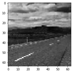
img, label = trainloader_small[0][0][40][0], trainloader_small[0][1][40]
label = int(np.array(label))
print(class_names[label])
imshow(img)
Highway
Problem 1: Training a Network From Scratch
{Part 1:} Gone are the days of hand designed features. Now we have end-to-end learning in which a highly non-linear representation is learned for our data to maximize our objective (in this case, 16-way classification accuracy). Instead of 70% accuracy we can now recognize scenes with… 25% accuracy. OK, that didn’t work at all. Try to boost the accuracy by doing the following:
Data Augmentation: We don’t have enough training data, let’s augment the training data. If you left-right flip (mirror) an image of a scene, it never changes categories. A kitchen doesn’t become a forest when mirrored. This isn’t true in all domains — a “d” becomes a “b” when mirrored, so you can’t “jitter” digit recognition training data in the same way. But we can synthetically increase our amount of training data by left-right mirroring training images during the learning process.
After you implement mirroring, you should notice that your training error doesn’t drop as quickly. That’s actually a good thing, because it means the network isn’t overfitting to the 2,400 original training images as much (because it sees 4,800 training images now, although they’re not as good as 4,800 truly independent samples). Because the training and test errors fall more slowly, you may need more training epochs or you may try modifying the learning rate. You should see a roughly 10% increase in accuracy by adding mirroring.
You can try more elaborate forms of jittering – zooming in a random amount, rotating a random amount, taking a random crop, etc. These are not required, you might want to try these in the bonus part.
Data Normalization: The images aren’t zero-centered. One simple trick which can help a lot is to subtract the mean from every image. It would arguably be more proper to only compute the mean from the training images (since the test/validation images should be strictly held out) but it won’t make much of a difference. After doing this you should see another 15% or so increase in accuracy.
Network Regularization: Add dropout layer. If you train your network (especially for more than the default 30 epochs) you’ll see that the training error can decrease to zero while the val top1 error hovers at 40% to 50%. The network has learned weights which can perfectly recognize the training data, but those weights don’t generalize to held out test data. The best regularization would be more training data but we don’t have that. Instead we will use dropout regularization.
What does dropout regularization do? It randomly turns off network connections at training time to fight overfitting. This prevents a unit in one layer from relying too strongly on a single unit in the previous layer. Dropout regularization can be interpreted as simultaneously training many “thinned” versions of your network. At test, all connections are restored which is analogous to taking an average prediction over all of the “thinned” networks. You can see a more complete discussion of dropout regularization in this paper.
The dropout layer has only one free parameter — the dropout rate — the proportion of connections that are randomly deleted. The default of 0.5 should be fine. Insert a dropout layer between your convolutional layers. In particular, insert it directly before your last convolutional layer. Your test accuracy should increase by another 10%. Your train accuracy should decrease much more slowly. That’s to be expected — you’re making life much harder for the training algorithm by cutting out connections randomly.
If you increase the number of training epochs (and maybe decrease the learning rate) you should be able to achieve around 50% test accuracy.
{Part 2:} Try three techniques taught in the class to increase the accuracy of your model. Such as increasing training data by randomly rotating training images, adding batch normalization, different activation functions (e.g., sigmoid) and model architecture modification. Note that too many layers can do you no good due to insufficient training data. Clearly describe your method and accuracy increase/decrease for each of the three techniques.
Part 1
# ==========================================
#       Define Network Architecture
# ==========================================
class ClassifierNetwork(nn.Module):

    def __init__(self, num_classes, d_out):
        super(ClassifierNetwork, self).__init__()

        # Convolution
        self.conv1 = nn.Conv2d(1, 32, kernel_size=3, stride=1, padding=1)
        self.relu1 = nn.ReLU()
        self.conv2 = nn.Conv2d(32, 64, kernel_size=3, stride=1, padding=1)
        self.relu2 = nn.ReLU()
        self.pool1 = torch.nn.MaxPool2d(kernel_size=2, stride=2, padding=0)
        self.d_out = nn.Dropout(d_out)
        self.conv3 = nn.Conv2d(64, 16, kernel_size=3, stride=1, padding=1)
        self.relu3 = nn.ReLU()
        self.pool2 = torch.nn.MaxPool2d(kernel_size=2, stride=2, padding=0)

        # Fully Connected Layers
        self.fc1 = nn.Linear(16 * 16 * 16, 64)
        self.fc2 = nn.Linear(64, 32)
        self.fc3 = nn.Linear(32, 16)

    def forward(self, x):
        y = self.conv1(x)
        y = self.relu1(y)
        y = self.conv2(y)
        y = self.relu2(y)
        y = self.pool1(y)
        y = self.d_out(y)
        y = self.conv3(y)
        y = self.relu3(y)
        y = self.pool2(y)
        y = y.view(y.size(0), -1)
        y = self.fc1(y)
        y = self.fc2(y)
        y = self.fc3(y)
        return y
# ==========================================
#         Optimize/Train Network
# ==========================================
def train(num_epochs, learning_rate, model, training_images, optimizer=None):
  if optimizer == None:
    optimizer = optim.Adam(model.parameters(), lr=learning_rate)

  criterion = nn.CrossEntropyLoss()

  since = time.time()
  # If GPU
  if torch.cuda.is_available():
      model = model.cuda()
      criterion = criterion.cuda()

  model.train()
  print(model)
  # print('Number of parameters: ', len(model.parameters()))

  total_step = len(training_images)
  print(total_step)
  loss_list = []
  acc_list = []

  for epoch in range(num_epochs):
      for i, (images, labels) in enumerate(training_images):
          if torch.cuda.is_available():
            # Move to GPU
            images, labels = images.cuda(), labels.cuda()

          # Run the forward pass
          outputs = model(images)
          loss = criterion(outputs, labels)
          loss_list.append(loss.item())

          # Backprop and perform Adam optimisation
          optimizer.zero_grad()
          loss.backward()
          optimizer.step()

          # Track the accuracy
          total = labels.size(0)
          _, predicted = torch.max(outputs.data, 1)
          correct = (predicted == labels).sum().item()
          acc_list.append(correct / total)

          if i != 0 and  i % (total_step - 1) == 0:
            print('Epoch [{}/{}], Step [{}/{}], Loss: {:.4f}, Accuracy: {:.2f}%'
                    .format(epoch + 1, num_epochs, i + 1, total_step, loss.item(),
                            (correct / total) * 100))

  elapsed = time.time() - since
  print('Train time elapsed in seconds: ', elapsed)
# Hyperparams
learning_rate = 0.001
num_epochs = 20

d_out = 0.5
num_classes = 16
model = ClassifierNetwork(num_classes, d_out)
train(num_epochs, learning_rate, model, trainloader_small)
ClassifierNetwork(
  (conv1): Conv2d(1, 32, kernel_size=(3, 3), stride=(1, 1), padding=(1, 1))
  (relu1): ReLU()
  (conv2): Conv2d(32, 64, kernel_size=(3, 3), stride=(1, 1), padding=(1, 1))
  (relu2): ReLU()
  (pool1): MaxPool2d(kernel_size=2, stride=2, padding=0, dilation=1, ceil_mode=False)
  (d_out): Dropout(p=0.5, inplace=False)
  (conv3): Conv2d(64, 16, kernel_size=(3, 3), stride=(1, 1), padding=(1, 1))
  (relu3): ReLU()
  (pool2): MaxPool2d(kernel_size=2, stride=2, padding=0, dilation=1, ceil_mode=False)
  (fc1): Linear(in_features=4096, out_features=64, bias=True)
  (fc2): Linear(in_features=64, out_features=32, bias=True)
  (fc3): Linear(in_features=32, out_features=16, bias=True)
)
96
Epoch [1/20], Step [96/96], Loss: 1.9985, Accuracy: 40.00%
Epoch [2/20], Step [96/96], Loss: 1.7693, Accuracy: 52.00%
Epoch [3/20], Step [96/96], Loss: 1.2488, Accuracy: 62.00%
Epoch [4/20], Step [96/96], Loss: 1.0325, Accuracy: 58.00%
Epoch [5/20], Step [96/96], Loss: 0.6761, Accuracy: 76.00%
Epoch [6/20], Step [96/96], Loss: 0.5512, Accuracy: 88.00%
Epoch [7/20], Step [96/96], Loss: 0.5590, Accuracy: 90.00%
Epoch [8/20], Step [96/96], Loss: 0.3916, Accuracy: 86.00%
Epoch [9/20], Step [96/96], Loss: 0.3435, Accuracy: 88.00%
Epoch [10/20], Step [96/96], Loss: 0.2134, Accuracy: 92.00%
Epoch [11/20], Step [96/96], Loss: 0.2164, Accuracy: 90.00%
Epoch [12/20], Step [96/96], Loss: 0.1143, Accuracy: 98.00%
Epoch [13/20], Step [96/96], Loss: 0.2784, Accuracy: 86.00%
Epoch [14/20], Step [96/96], Loss: 0.1736, Accuracy: 92.00%
Epoch [15/20], Step [96/96], Loss: 0.1165, Accuracy: 98.00%
Epoch [16/20], Step [96/96], Loss: 0.0692, Accuracy: 96.00%
Epoch [17/20], Step [96/96], Loss: 0.1048, Accuracy: 96.00%
Epoch [18/20], Step [96/96], Loss: 0.0841, Accuracy: 98.00%
Epoch [19/20], Step [96/96], Loss: 0.0597, Accuracy: 100.00%
Epoch [20/20], Step [96/96], Loss: 0.0273, Accuracy: 98.00%
Train time elapsed in seconds:  68.62133049964905
# ==========================================
#            Evaluating Network
# ==========================================
# Test the model
def test(model, test_images):
  since = time.time()
  model.eval()
  with torch.no_grad():
      correct = 0
      total = 0
      for images, labels in test_images:
          if torch.cuda.is_available():
            # Move to GPU
            images, labels = images.cuda(), labels.cuda()

          outputs = model(images)
          _, predicted = torch.max(outputs.data, 1)
          total += labels.size(0)
          correct += (predicted == labels).sum().item()

      print('Test Accuracy of the model on test images: {} %'.format((correct / total) * 100))

  elapsed = time.time() - since
  print('Test time elapsed in seconds: ', elapsed)
test(model, testloader_small)
Test Accuracy of the model on test images: 53.0 %
Test time elapsed in seconds:  0.0289766788482666
# Save the model
# torch.save(model.state_dict(), 'simple_5300_conv_net_model_{}.ckpt'.format(time.time()))
Pre-Processing
Data augmentation:
As part of the data augmentation, we horizontally flip each of the training images. This helps us generate 2400 more images to add to our existing training images. Tests images are not flipped.
Data normalization:
As part of the data normalization we subtract the mean of all the images from each image. This helps with zero-centering all our images. Both train and test images are normazlied.
Network Regularization:
We implement dropout in our CNN architecture to regularize the network and ensure it does not overfit our training images. Using a dropout rate of 0.5.
CNN ARCHITECTURE:
CNN Layers:
- Layer 1: Convolution 1 (conv1): 1 input channel, 32 output channels, 3x3 kernels, 1px stride, 1px padding
Relu 1 (relu1) - Layer 3: Convolution 2 (conv2): 32 input channels, 64 output channels, 3x3 kernels, 1px stride, 1px padding
Relu 2 (relu2)
Max Pooling 1 (pool1): 2x2 kernel, 2px stride, 0px padding - Dropout (d_out): 0.5 dropout rate
- Convolution 3 (conv3): 64 input channels, 16 output channels, 3x3 kernels, 1px stride, 1px padding
Relu 3 (relu3)
Max Pooling 1 (pool1): 2x2 kernel, 2px stride, 0px padding
Fully Connected Layers:
- FC Layer 1 (fc1): in_features=4096, out_features=64, bias=True
- FC Layer 2 (fc2): in_features=64, out_features=32, bias=True
- FC Layer 3 (fc3): in_features=32, out_features=16, bias=True
Model Parameters:
- Number of Epochs: 20
- Learning Rate: 0.001
- Optimizer: Adam
- Loss Function: Cross Entropy Loss
Model Performance:
- Training time: ~70s
- Test (Evaluation) time: <1s
- Accuracy: ~53% to ~55%
NOTE: Model training time and accuracy fluctuate a bit because of random initialization of weight in each run but is consistently above 50%, sometimes reaching 59%.
Part 2
Variation 1 - Use Sigmoid instead of ReLU as our activation function across our network from Part 1.
# ==========================================
#       Same Network with Sigmoid
# ==========================================
class ClassifierNetworkSigmoid(nn.Module):

    def __init__(self, num_classes, d_out):
      super(ClassifierNetworkSigmoid, self).__init__()

      # Convolution
      self.conv1 = nn.Conv2d(1, 32, kernel_size=3, stride=1, padding=1)
      self.sigm1 = nn.Sigmoid()
      self.conv2 = nn.Conv2d(32, 64, kernel_size=3, stride=1, padding=1)
      self.sigm2 = nn.Sigmoid()
      self.pool1 = torch.nn.MaxPool2d(kernel_size=2, stride=2, padding=0)
      self.d_out = nn.Dropout(d_out)
      self.conv3 = nn.Conv2d(64, 16, kernel_size=3, stride=1, padding=1)
      self.sigm3 = nn.Sigmoid()
      self.pool2 = torch.nn.MaxPool2d(kernel_size=2, stride=2, padding=0)

      # Fully Connected Layers
      self.fc1 = nn.Linear(16 * 16 * 16, 64)
      self.fc2 = nn.Linear(64, 32)
      self.fc3 = nn.Linear(32, 16)

    def forward(self, x):
      y = self.conv1(x)
      y = self.sigm1(y)
      y = self.conv2(y)
      y = self.sigm2(y)
      y = self.pool1(y)
      y = self.d_out(y)
      y = self.conv3(y)
      y = self.sigm3(y)
      y = self.pool2(y)
      y = y.view(y.size(0), -1)
      y = self.fc1(y)
      y = self.fc2(y)
      y = self.fc3(y)
      return y
sigm_model = ClassifierNetworkSigmoid(num_classes, d_out)
train(num_epochs, learning_rate, sigm_model, trainloader_small)
ClassifierNetworkSigmoid(
  (conv1): Conv2d(1, 32, kernel_size=(3, 3), stride=(1, 1), padding=(1, 1))
  (sigm1): Sigmoid()
  (conv2): Conv2d(32, 64, kernel_size=(3, 3), stride=(1, 1), padding=(1, 1))
  (sigm2): Sigmoid()
  (pool1): MaxPool2d(kernel_size=2, stride=2, padding=0, dilation=1, ceil_mode=False)
  (d_out): Dropout(p=0.5, inplace=False)
  (conv3): Conv2d(64, 16, kernel_size=(3, 3), stride=(1, 1), padding=(1, 1))
  (sigm3): Sigmoid()
  (pool2): MaxPool2d(kernel_size=2, stride=2, padding=0, dilation=1, ceil_mode=False)
  (fc1): Linear(in_features=4096, out_features=64, bias=True)
  (fc2): Linear(in_features=64, out_features=32, bias=True)
  (fc3): Linear(in_features=32, out_features=16, bias=True)
)
96
Epoch [1/20], Step [96/96], Loss: 2.7894, Accuracy: 2.00%
Epoch [2/20], Step [96/96], Loss: 2.7803, Accuracy: 2.00%
Epoch [3/20], Step [96/96], Loss: 2.7732, Accuracy: 8.00%
Epoch [4/20], Step [96/96], Loss: 2.7347, Accuracy: 10.00%
Epoch [5/20], Step [96/96], Loss: 2.4545, Accuracy: 18.00%
Epoch [6/20], Step [96/96], Loss: 2.3884, Accuracy: 28.00%
Epoch [7/20], Step [96/96], Loss: 2.3561, Accuracy: 30.00%
Epoch [8/20], Step [96/96], Loss: 2.3131, Accuracy: 28.00%
Epoch [9/20], Step [96/96], Loss: 2.2976, Accuracy: 26.00%
Epoch [10/20], Step [96/96], Loss: 2.2014, Accuracy: 32.00%
Epoch [11/20], Step [96/96], Loss: 1.8794, Accuracy: 42.00%
Epoch [12/20], Step [96/96], Loss: 1.6576, Accuracy: 50.00%
Epoch [13/20], Step [96/96], Loss: 1.4731, Accuracy: 60.00%
Epoch [14/20], Step [96/96], Loss: 1.4460, Accuracy: 56.00%
Epoch [15/20], Step [96/96], Loss: 1.3027, Accuracy: 62.00%
Epoch [16/20], Step [96/96], Loss: 1.2590, Accuracy: 56.00%
Epoch [17/20], Step [96/96], Loss: 1.0755, Accuracy: 58.00%
Epoch [18/20], Step [96/96], Loss: 0.9489, Accuracy: 76.00%
Epoch [19/20], Step [96/96], Loss: 0.8910, Accuracy: 78.00%
Epoch [20/20], Step [96/96], Loss: 0.8051, Accuracy: 80.00%
Train time elapsed in seconds:  69.16449451446533
test(sigm_model, testloader_small)
Test Accuracy of the model on test images: 42.75 %
Test time elapsed in seconds:  0.0942375659942627
Variation 2 - Use of Batch Normalization
# ==========================================
# Same Network with Intermediate Batch Norm
# ==========================================
class ClassifierNetworkBatchNorm(nn.Module):

    def __init__(self, num_classes, d_out):
      super(ClassifierNetworkBatchNorm, self).__init__()

      # Convolution
      self.conv1 = nn.Conv2d(1, 32, kernel_size=3, stride=1, padding=1)
      self.relu1 = nn.ReLU()
      self.conv2 = nn.Conv2d(32, 64, kernel_size=3, stride=1, padding=1)
      self.conv2_bn = nn.BatchNorm2d(64)
      self.relu2 = nn.ReLU()
      self.pool1 = torch.nn.MaxPool2d(kernel_size=2, stride=2, padding=0)
      self.d_out = nn.Dropout(d_out)
      self.conv3 = nn.Conv2d(64, 16, kernel_size=3, stride=1, padding=1)
      self.conv3_bn = nn.BatchNorm2d(16)
      self.relu3 = nn.ReLU()
      self.pool2 = torch.nn.MaxPool2d(kernel_size=2, stride=2, padding=0)

      # Fully Connected Layers
      self.fc1 = nn.Linear(16 * 16 * 16, 64)
      self.fc2 = nn.Linear(64, 32)
      self.fc2_bn = nn.BatchNorm1d(32)
      self.fc3 = nn.Linear(32, 16)

    def forward(self, x):
      y = self.conv1(x)
      y = self.relu1(y)
      y = self.conv2(y)
      y = self.conv2_bn(y)
      y = self.relu2(y)
      y = self.pool1(y)
      y = self.d_out(y)
      y = self.conv3(y)
      y = self.conv3_bn(y)
      y = self.relu3(y)
      y = self.pool2(y)
      y = y.view(y.size(0), -1)
      y = self.fc1(y)
      y = self.fc2(y)
      y = self.fc2_bn(y)
      y = self.fc3(y)
      return y
bn_model = ClassifierNetworkBatchNorm(num_classes, d_out)
train(num_epochs, learning_rate, bn_model, trainloader_small)
test(bn_model, testloader_small)
ClassifierNetworkBatchNorm(
  (conv1): Conv2d(1, 32, kernel_size=(3, 3), stride=(1, 1), padding=(1, 1))
  (relu1): ReLU()
  (conv2): Conv2d(32, 64, kernel_size=(3, 3), stride=(1, 1), padding=(1, 1))
  (conv2_bn): BatchNorm2d(64, eps=1e-05, momentum=0.1, affine=True, track_running_stats=True)
  (relu2): ReLU()
  (pool1): MaxPool2d(kernel_size=2, stride=2, padding=0, dilation=1, ceil_mode=False)
  (d_out): Dropout(p=0.5, inplace=False)
  (conv3): Conv2d(64, 16, kernel_size=(3, 3), stride=(1, 1), padding=(1, 1))
  (conv3_bn): BatchNorm2d(16, eps=1e-05, momentum=0.1, affine=True, track_running_stats=True)
  (relu3): ReLU()
  (pool2): MaxPool2d(kernel_size=2, stride=2, padding=0, dilation=1, ceil_mode=False)
  (fc1): Linear(in_features=4096, out_features=64, bias=True)
  (fc2): Linear(in_features=64, out_features=32, bias=True)
  (fc2_bn): BatchNorm1d(32, eps=1e-05, momentum=0.1, affine=True, track_running_stats=True)
  (fc3): Linear(in_features=32, out_features=16, bias=True)
)
96
Epoch [1/20], Step [96/96], Loss: 1.7865, Accuracy: 44.00%
Epoch [2/20], Step [96/96], Loss: 1.2338, Accuracy: 70.00%
Epoch [3/20], Step [96/96], Loss: 0.8534, Accuracy: 70.00%
Epoch [4/20], Step [96/96], Loss: 0.5359, Accuracy: 88.00%
Epoch [5/20], Step [96/96], Loss: 0.3470, Accuracy: 98.00%
Epoch [6/20], Step [96/96], Loss: 0.2767, Accuracy: 98.00%
Epoch [7/20], Step [96/96], Loss: 0.2840, Accuracy: 96.00%
Epoch [8/20], Step [96/96], Loss: 0.1737, Accuracy: 100.00%
Epoch [9/20], Step [96/96], Loss: 0.1066, Accuracy: 100.00%
Epoch [10/20], Step [96/96], Loss: 0.0683, Accuracy: 100.00%
Epoch [11/20], Step [96/96], Loss: 0.1027, Accuracy: 100.00%
Epoch [12/20], Step [96/96], Loss: 0.0328, Accuracy: 100.00%
Epoch [13/20], Step [96/96], Loss: 0.0736, Accuracy: 100.00%
Epoch [14/20], Step [96/96], Loss: 0.0462, Accuracy: 100.00%
Epoch [15/20], Step [96/96], Loss: 0.0195, Accuracy: 100.00%
Epoch [16/20], Step [96/96], Loss: 0.0374, Accuracy: 100.00%
Epoch [17/20], Step [96/96], Loss: 0.0241, Accuracy: 100.00%
Epoch [18/20], Step [96/96], Loss: 0.0163, Accuracy: 100.00%
Epoch [19/20], Step [96/96], Loss: 0.0115, Accuracy: 100.00%
Epoch [20/20], Step [96/96], Loss: 0.0105, Accuracy: 100.00%
Train time elapsed in seconds:  76.71598410606384
Test Accuracy of the model on test images: 60.25 %
Test time elapsed in seconds:  0.09820342063903809
Variation 3: Adding more augmented data (slightly rotated images)
# Augmenting dataset for this variation to have more images which are slightly rotated.

# load data into size (64, 64)
img_size = (64, 64)
batch_num = 50 # training sample number per batch

# load training dataset
trainloader_small_rot = list(load_dataset('./data/train/', img_size, batch_num=batch_num, shuffle=True,
                                      augment=True, zero_centered=True, rotate=10))
train_num = len(trainloader_small)
print("Finish loading %d minibatches(=%d) of training samples." % (train_num, batch_num))
Loading images from class: 0
Loading images from class: 1
Loading images from class: 2
Loading images from class: 3
Loading images from class: 4
Loading images from class: 5
Loading images from class: 6
Loading images from class: 7
Loading images from class: 8
Loading images from class: 9
Loading images from class: 10
Loading images from class: 11
Loading images from class: 12
Loading images from class: 13
Loading images from class: 14
Loading images from class: 15
Augmenting data by horizontally flipping them!
Total flipped images:  2400
Total data before flipped images:  2400
Total data after adding horizontally flipped images:  4800
(64, 64)
Augmenting data by randomly rotating them!
Total rotated images:  4800
Total data before rotated images:  4800
Total data after adding rotated images:  9600
9600
50
Finish loading 96 minibatches(=50) of training samples.
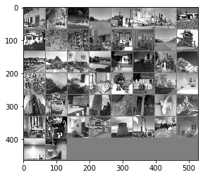
# Get a batch of training data
inputs, classes = next(iter(trainloader_small_rot))

# Make a grid from batch
out = torchvision.utils.make_grid(inputs)

imshow(out)
Clipping input data to the valid range for imshow with RGB data ([0..1] for floats or [0..255] for integers).
rot_model = ClassifierNetwork(num_classes, d_out)
train(num_epochs, learning_rate, rot_model, trainloader_small_rot)
test(rot_model, testloader_small)
ClassifierNetwork(
  (conv1): Conv2d(1, 32, kernel_size=(3, 3), stride=(1, 1), padding=(1, 1))
  (relu1): ReLU()
  (conv2): Conv2d(32, 64, kernel_size=(3, 3), stride=(1, 1), padding=(1, 1))
  (relu2): ReLU()
  (pool1): MaxPool2d(kernel_size=2, stride=2, padding=0, dilation=1, ceil_mode=False)
  (d_out): Dropout(p=0.5, inplace=False)
  (conv3): Conv2d(64, 16, kernel_size=(3, 3), stride=(1, 1), padding=(1, 1))
  (relu3): ReLU()
  (pool2): MaxPool2d(kernel_size=2, stride=2, padding=0, dilation=1, ceil_mode=False)
  (fc1): Linear(in_features=4096, out_features=64, bias=True)
  (fc2): Linear(in_features=64, out_features=32, bias=True)
  (fc3): Linear(in_features=32, out_features=16, bias=True)
)
192
Epoch [1/20], Step [192/192], Loss: 1.8327, Accuracy: 46.00%
Epoch [2/20], Step [192/192], Loss: 1.3683, Accuracy: 52.00%
Epoch [3/20], Step [192/192], Loss: 1.0431, Accuracy: 66.00%
Epoch [4/20], Step [192/192], Loss: 0.6368, Accuracy: 74.00%
Epoch [5/20], Step [192/192], Loss: 0.4520, Accuracy: 84.00%
Epoch [6/20], Step [192/192], Loss: 0.2821, Accuracy: 90.00%
Epoch [7/20], Step [192/192], Loss: 0.2657, Accuracy: 88.00%
Epoch [8/20], Step [192/192], Loss: 0.1120, Accuracy: 96.00%
Epoch [9/20], Step [192/192], Loss: 0.1282, Accuracy: 94.00%
Epoch [10/20], Step [192/192], Loss: 0.1870, Accuracy: 94.00%
Epoch [11/20], Step [192/192], Loss: 0.6496, Accuracy: 82.00%
Epoch [12/20], Step [192/192], Loss: 0.2355, Accuracy: 92.00%
Epoch [13/20], Step [192/192], Loss: 0.0194, Accuracy: 100.00%
Epoch [14/20], Step [192/192], Loss: 0.1474, Accuracy: 94.00%
Epoch [15/20], Step [192/192], Loss: 0.0611, Accuracy: 98.00%
Epoch [16/20], Step [192/192], Loss: 0.0207, Accuracy: 100.00%
Epoch [17/20], Step [192/192], Loss: 0.0491, Accuracy: 98.00%
Epoch [18/20], Step [192/192], Loss: 0.1151, Accuracy: 96.00%
Epoch [19/20], Step [192/192], Loss: 0.0606, Accuracy: 98.00%
Epoch [20/20], Step [192/192], Loss: 0.1107, Accuracy: 96.00%
Train time elapsed in seconds:  137.09119653701782
Test Accuracy of the model on test images: 52.0 %
Test time elapsed in seconds:  0.09217381477355957
Note: Across these variations, we stick to the same number of epochs (20), learning rate (0.0001), optimizer (Adam) and loss function (Cross Entropy) like we used in our simple CNN model. This makes it easy to compare our accuracies with the variations with our simple CNN model.
Variation 1:
-
In this variation we only change the activation function used from ReLU to Sigmoid across the model. From eyeballing the accuracies we notice that this variation is slow to start off the block but does manage to increase accuracy in further epochs. Eventually it does fall short of our original model in terms of accuracy on the test images. Training accuracy does not peak in the 20 epochs that we had set, which gives us reason to believe that there is room for the model to learn if we increse the number of epochs.
- Training time: ~70s
- Test (Evaluation) time: <1s
- Accuracy: ~40% to ~43%
Variation 2:
-
In this variation we add a couple of batch normalization layers after our 2nd and 3rd convolution layers and our second fully connected layer. This is done to ensure our intermediate layers do not depend too much on the variation of the values produced by their preceding layers. Eyeballing the accuracies across the epochs one can notice that we reach training accuracy of 100% in almost 10 epochs itself. This gives us reason to believe that we might be overfitting our model by training further. We do get slightly better accuracy (around 2-3%) with this model, but this could possibly be bettered if we decrease the number of epochs in order to verify our claim of overfitting.
- Training time: ~75s
- Test (Evaluation) time: <1s
- Accuracy: ~55% to ~60%
Variation 3:
-
In this variation we try to add more augmented data by randomly rotating images within a certain angle range (10 degress). This takes our training dataset size to 9600. This does not seem to help increase the final accuracy too much but one can notice that our training accuracy reaches higher values much faster than our simple CNN model. We have given our model more images to train but given they are very similar it is learning them faster. But this does not help on our test images as we seem to be performing relatively at par with our somple CNN model.
- Training time: ~140s
- Test (Evaluation) time: <1s
- Accuracy: ~55% to ~58%
Problem 2: Fine Tuning a Pre-Trained Deep Network
{Part 1:} Our convolutional network to this point isn’t “deep”. Fortunately, the representations learned by deep convolutional networks is that they generalize surprisingly well to other recognition tasks.
But how do we use an existing deep network for a new recognition task? Take for instance, AlexNet network has 1000 units in the final layer corresponding to 1000 ImageNet categories.
Strategy A: One could use those 1000 activations as a feature in place of a hand crafted feature such as a bag-of-features representation. You would train a classifier (typically a linear SVM) in that 1000 dimensional feature space. However, those activations are clearly very object specific and may not generalize well to new recognition tasks. It is generally better to use the activations in slightly earlier layers of the network, e.g. the 4096 activations in the last 2nd fully-connected layer. You can often get away with sub-sampling those 4096 activations considerably, e.g. taking only the first 200 activations.
Strategy B: Fine-tune an existing network. In this scenario you take an existing network, replace the final layer (or more) with random weights, and train the entire network again with images and ground truth labels for your recognition task. You are effectively treating the pre-trained deep network as a better initialization than the random weights used when training from scratch. When you don’t have enough training data to train a complex network from scratch (e.g. with the 16 classes) this is an attractive option. Fine-tuning can work far better than Strategy A of taking the activations directly from an pre-trained CNN. For example, in this paper from CVPR 2015, there wasn’t enough data to train a deep network from scratch, but fine tuning led to 4 times higher accuracy than using off-the-shelf networks directly.
We implement Strategy B to fine-tune a pre-trained AlexNet for this scene classification task. You should be able to achieve performance of 85% approximately. It takes roughly 35~40 minutes to train 20 epoches with AlexNet.
Detailed descriptions of these present below:
(1) which layers of AlexNet have been replaced
(2) the architecture of the new layers added including activation methods (same as problem 1)
(3) the final accuracy on test set along with time consumption for both training and testing
{Part 2:} Implement Strategy A where you use the activations of the pre-trained network as features to train one-vs-all SVMs for your scene classification task. Report the final accuracy on test set along with time consumption for both training and testing.
We also fine-tune the VGG network paper and compare performance with AlexNet.
Hints:
- Many pre-trained models are available in PyTorch at here.
- For fine-tuning pretrained network using PyTorch, please read this tutorial.
Load Images
# reload data with a larger size
img_size = (224, 224)
batch_num = 50 # training sample number per batch

# load training dataset
trainloader_large = list(load_dataset('./data/train/', img_size, batch_num=batch_num, shuffle=True,
                                      augment=False, is_color=True, zero_centered=True))
train_num = len(trainloader_large)
print("Finish loading %d minibatches(=%d) of training samples." % (train_num, batch_num))

# load testing dataset
testloader_large = list(load_dataset('./data/test/', img_size, num_per_class=50, batch_num=batch_num, is_color=True))
test_num = len(testloader_large)
print("Finish loading %d minibatches(=%d) of testing samples." % (test_num, batch_num))
Loading images from class: 0
Loading images from class: 1
Loading images from class: 2
Loading images from class: 3
Loading images from class: 4
Loading images from class: 5
Loading images from class: 6
Loading images from class: 7
Loading images from class: 8
Loading images from class: 9
Loading images from class: 10
Loading images from class: 11
Loading images from class: 12
Loading images from class: 13
Loading images from class: 14
Loading images from class: 15
(3, 224, 224)
2400
50
Finish loading 48 minibatches(=50) of training samples.
Loading images from class: 0
Loading images from class: 1
Loading images from class: 2
Loading images from class: 3
Loading images from class: 4
Loading images from class: 5
Loading images from class: 6
Loading images from class: 7
Loading images from class: 8
Loading images from class: 9
Loading images from class: 10
Loading images from class: 11
Loading images from class: 12
Loading images from class: 13
Loading images from class: 14
Loading images from class: 15
400
50
Finish loading 8 minibatches(=50) of testing samples.
Strategy B Implementation
# ==========================================
#       Fine-Tune Pretrained Network
# ==========================================
alexnet = models.alexnet(pretrained=True)
# alexnet.features[0] = nn.Conv2d(3, 64, kernel_size=7, stride=4, padding=2)
alexnet.classifier[6] = nn.Linear(4096, 16)
# alexnet_mod = nn.Sequential(alexnet, nn.Linear(1024, 16))
# alexnet = models.alexnet(num_classes=16)

alexnet_num_epochs = 20
alexnet_learning_rate = 0.0001

train(alexnet_num_epochs, alexnet_learning_rate, alexnet, trainloader_large)
test(alexnet, testloader_large)
AlexNet(
  (features): Sequential(
    (0): Conv2d(3, 64, kernel_size=(11, 11), stride=(4, 4), padding=(2, 2))
    (1): ReLU(inplace=True)
    (2): MaxPool2d(kernel_size=3, stride=2, padding=0, dilation=1, ceil_mode=False)
    (3): Conv2d(64, 192, kernel_size=(5, 5), stride=(1, 1), padding=(2, 2))
    (4): ReLU(inplace=True)
    (5): MaxPool2d(kernel_size=3, stride=2, padding=0, dilation=1, ceil_mode=False)
    (6): Conv2d(192, 384, kernel_size=(3, 3), stride=(1, 1), padding=(1, 1))
    (7): ReLU(inplace=True)
    (8): Conv2d(384, 256, kernel_size=(3, 3), stride=(1, 1), padding=(1, 1))
    (9): ReLU(inplace=True)
    (10): Conv2d(256, 256, kernel_size=(3, 3), stride=(1, 1), padding=(1, 1))
    (11): ReLU(inplace=True)
    (12): MaxPool2d(kernel_size=3, stride=2, padding=0, dilation=1, ceil_mode=False)
  )
  (avgpool): AdaptiveAvgPool2d(output_size=(6, 6))
  (classifier): Sequential(
    (0): Dropout(p=0.5, inplace=False)
    (1): Linear(in_features=9216, out_features=4096, bias=True)
    (2): ReLU(inplace=True)
    (3): Dropout(p=0.5, inplace=False)
    (4): Linear(in_features=4096, out_features=4096, bias=True)
    (5): ReLU(inplace=True)
    (6): Linear(in_features=4096, out_features=16, bias=True)
  )
)
48
Epoch [1/20], Step [48/48], Loss: 0.3987, Accuracy: 88.00%
Epoch [2/20], Step [48/48], Loss: 0.2584, Accuracy: 90.00%
Epoch [3/20], Step [48/48], Loss: 0.0922, Accuracy: 98.00%
Epoch [4/20], Step [48/48], Loss: 0.1944, Accuracy: 96.00%
Epoch [5/20], Step [48/48], Loss: 0.0306, Accuracy: 100.00%
Epoch [6/20], Step [48/48], Loss: 0.1302, Accuracy: 94.00%
Epoch [7/20], Step [48/48], Loss: 0.0041, Accuracy: 100.00%
Epoch [8/20], Step [48/48], Loss: 0.0322, Accuracy: 100.00%
Epoch [9/20], Step [48/48], Loss: 0.0271, Accuracy: 100.00%
Epoch [10/20], Step [48/48], Loss: 0.0088, Accuracy: 100.00%
Epoch [11/20], Step [48/48], Loss: 0.0170, Accuracy: 100.00%
Epoch [12/20], Step [48/48], Loss: 0.0385, Accuracy: 100.00%
Epoch [13/20], Step [48/48], Loss: 0.0010, Accuracy: 100.00%
Epoch [14/20], Step [48/48], Loss: 0.0032, Accuracy: 100.00%
Epoch [15/20], Step [48/48], Loss: 0.0073, Accuracy: 100.00%
Epoch [16/20], Step [48/48], Loss: 0.0103, Accuracy: 100.00%
Epoch [17/20], Step [48/48], Loss: 0.0070, Accuracy: 100.00%
Epoch [18/20], Step [48/48], Loss: 0.0020, Accuracy: 100.00%
Epoch [19/20], Step [48/48], Loss: 0.0009, Accuracy: 100.00%
Epoch [20/20], Step [48/48], Loss: 0.0148, Accuracy: 100.00%
Train time elapsed in seconds:  125.99178218841553
Test Accuracy of the model on test images: 84.5 %
Test time elapsed in seconds:  0.30092597007751465
Change in AlexNet:
Only the last layer of the network was changed. Instead of the linear layer from 4096 input features to 1000 output features in the original AlexNet architecture, we change it to 16 output features for the purpose of this classification.
Note: Other change tried (but commented out) did NOT seem to help increase accuracy.
-
Tried adding one more fully connected layer to change to look like 4096 -> 1024 -> 16 instead of 4096 -> 16. This increased training time, as expected, but dropped accuracy by a couple of percents.
-
Tried changing the kernel size for the first convolution to 7x7 instead of 11x11. This too dropped accuracy instead.
Final AlexNet architecture:
- Layer 1: Convolution 1 (conv1): 3 input channel, 64 output channels, 11x11 kernels, 4px stride, 2px padding
- Relu 1 (relu1)
- Max Pooling 1 (pool1): 3x3 kernel, 2px stride, 0px padding
- Layer 2: Convolution 2 (conv2): 64 input channel, 192 output channels, 5x5 kernels, 1px stride, 2px padding
- Relu 2 (relu2)
- Max Pooling 2 (pool2): 3x3 kernel, 2px stride, 0px padding
- Layer 3: Convolution 3 (conv3): 192 input channels, 384 output channels, 3x3 kernels, 1px stride, 1px padding
- Relu 3 (relu3)
- Layer 4: Convolution 4 (conv4): 384 input channels, 256 output channels, 3x3 kernels, 1px stride, 1px padding
- Relu 4 (relu4)
- Layer 5: Convolution 5 (conv3): 256 input channels, 256 output channels, 3x3 kernels, 1px stride, 1px padding
- Relu 5 (relu5)
- Max Pooling 3 (pool3): 3x3 kernel, 2px stride, 0px padding
- Layer 6: Adaptive Avg Pool (avgpool): output: 6x6
- Dropout (d_out): 0.5 dropout rate
- FC Layer 1 (fc1): in_features=9216, out_features=4096
- Relu 6 (relu6)
- Dropout (d_out): 0.5 dropout rate
- FC Layer 2 (fc2): in_features=4096, out_features=4096
- Relu 7 (relu7)
- FC Layer 3 (fc3): in_features=4096, out_features=16
Model Performance:
- Training time: ~120s to ~125s
- Test (Evaluation) time: <1s
- Accuracy: ~84% to ~86%
# torch.save(alexnet.state_dict(), 'alexnet_{}_fine_tune_model_{}.ckpt'.format('add_accuracy_here',time.time()))
Strategy A Implementation
# ==========================================
#  Freeze weights for Pretrained Network
# ==========================================
alexnet_ft = models.alexnet(pretrained=True)

# Disable gradient calculations and freeze weights
for param in alexnet_ft.parameters():
    param.requires_grad = False

print(alexnet_ft)
AlexNet(
  (features): Sequential(
    (0): Conv2d(3, 64, kernel_size=(11, 11), stride=(4, 4), padding=(2, 2))
    (1): ReLU(inplace=True)
    (2): MaxPool2d(kernel_size=3, stride=2, padding=0, dilation=1, ceil_mode=False)
    (3): Conv2d(64, 192, kernel_size=(5, 5), stride=(1, 1), padding=(2, 2))
    (4): ReLU(inplace=True)
    (5): MaxPool2d(kernel_size=3, stride=2, padding=0, dilation=1, ceil_mode=False)
    (6): Conv2d(192, 384, kernel_size=(3, 3), stride=(1, 1), padding=(1, 1))
    (7): ReLU(inplace=True)
    (8): Conv2d(384, 256, kernel_size=(3, 3), stride=(1, 1), padding=(1, 1))
    (9): ReLU(inplace=True)
    (10): Conv2d(256, 256, kernel_size=(3, 3), stride=(1, 1), padding=(1, 1))
    (11): ReLU(inplace=True)
    (12): MaxPool2d(kernel_size=3, stride=2, padding=0, dilation=1, ceil_mode=False)
  )
  (avgpool): AdaptiveAvgPool2d(output_size=(6, 6))
  (classifier): Sequential(
    (0): Dropout(p=0.5, inplace=False)
    (1): Linear(in_features=9216, out_features=4096, bias=True)
    (2): ReLU(inplace=True)
    (3): Dropout(p=0.5, inplace=False)
    (4): Linear(in_features=4096, out_features=4096, bias=True)
    (5): ReLU(inplace=True)
    (6): Linear(in_features=4096, out_features=1000, bias=True)
  )
)
# ==========================================
#  Extract Features using last layer of n/w
# ==========================================

def extract_features(model, num_features, image_batches):
  model.eval()
  if torch.cuda.is_available():
      model = model.cuda()

  x = []
  y = []
  for i, (images, labels) in enumerate(image_batches):
    if torch.cuda.is_available():
      images, labels = images.cuda(), labels.cuda()

    outputs = model(images)

    for index, output in enumerate(outputs):
      # print(output[:num_features].cpu().detach().numpy())
      x.append(np.array(output[:num_features].cpu().detach().numpy()))
      y.append(labels[index].cpu().detach().numpy())

  return np.array(x), np.array(y)

num_features = 400
X_train, y_train = extract_features(alexnet_ft, num_features, trainloader_large)
# print(X_train, y_train)
print(len(X_train), len(y_train))
X_test, y_test = extract_features(alexnet_ft, num_features, testloader_large)
print(len(X_test), len(y_test))
# for img, lab in dat[:2]:
#   print(img, lab)
2400 2400
400 400
# ==========================================
#  Train LinearSVC one-vs-all
# ==========================================
lin_clf = svm.LinearSVC(C=0.001)
since = time.time()
lin_clf.fit(X_train, y_train)
elapsed = time.time() - since
print('Train time elapsed in seconds: ', elapsed)
Train time elapsed in seconds: 0.9073934555053711
# ==========================================
#  Test on LinearSVC
# ==========================================
since = time.time()
y_pred = lin_clf.predict(X_test)
elapsed = time.time() - since
print('Test time elapsed in seconds: ', elapsed)
cm = confusion_matrix(y_test, y_pred)
print('Accuracy using {} feature points from last layer of pretrained AlexNext is {}%'.
      format(num_features, accuracy_score(y_test, y_pred)*100))

print(cm)
Test time elapsed in seconds:  0.0026221275329589844
Accuracy using 400 feature points from last layer of pretrained AlexNext is 85.25%
[[25  0  0  0  0  0  0  0  0  0  0  0  0  0  0  0]
 [ 0 20  0  0  0  0  0  0  0  0  2  1  2  0  0  0]
 [ 0  0 21  0  0  0  0  0  1  3  0  0  0  0  0  0]
 [ 0  0  0 24  0  1  0  0  0  0  0  0  0  0  0  0]
 [ 0  5  0  0 20  0  0  0  0  0  0  0  0  0  0  0]
 [ 0  0  0  0  0 22  0  0  1  0  0  0  0  2  0  0]
 [ 0  0  0  0  0  0 22  0  0  2  0  0  0  1  0  0]
 [ 0  0  1  0  0  0  0 17  0  3  0  0  0  0  0  4]
 [ 1  0  3  0  0  0  0  0 18  1  0  0  0  2  0  0]
 [ 0  0  1  0  0  0  0  4  0 18  0  0  0  0  0  2]
 [ 0  0  0  0  0  0  0  0  0  0 25  0  0  0  0  0]
 [ 0  0  0  0  0  0  0  0  0  0  0 25  0  0  0  0]
 [ 0  2  0  0  1  0  0  0  0  0  1  0 21  0  0  0]
 [ 0  0  2  1  0  2  0  0  0  0  0  0  0 19  0  1]
 [ 0  0  0  0  0  0  0  0  0  0  0  0  0  0 25  0]
 [ 0  0  0  0  0  0  0  5  0  0  0  0  0  1  0 19]]
We use a Linear SVC for classifying based on output representations of images on pretrained model of AlexNet. We ensure we do not update gradients of the model during the forward pass of the model to get output representations. The lambda or the regularization factor for the Linear SVC is 0.001.
We use sample only the first 400 features from the 1000 features output of the AlexNet for classifications. We managed to get an accuracy of around 85.25% using our LinearSVC. The confusion matrix also looks pretty decent with higher numbers on the diagonal elements.
Training and test time are neglible, less than 1s, for our small dataset.
NOTE: Using 200 features (as suggested in the assignment) we could not match the same accuracy we received for Strategy B.
Bonus: VGG
vgg16 = models.vgg16(pretrained=True)
vgg16.classifier[6] = nn.Linear(4096, 16)
print(vgg16)

vgg16_num_epochs = 20
vgg16_learning_rate = 0.0001

train(vgg16_num_epochs, vgg16_learning_rate, vgg16, trainloader_large)
test(vgg16, testloader_large)
VGG(
  (features): Sequential(
    (0): Conv2d(3, 64, kernel_size=(3, 3), stride=(1, 1), padding=(1, 1))
    (1): ReLU(inplace=True)
    (2): Conv2d(64, 64, kernel_size=(3, 3), stride=(1, 1), padding=(1, 1))
    (3): ReLU(inplace=True)
    (4): MaxPool2d(kernel_size=2, stride=2, padding=0, dilation=1, ceil_mode=False)
    (5): Conv2d(64, 128, kernel_size=(3, 3), stride=(1, 1), padding=(1, 1))
    (6): ReLU(inplace=True)
    (7): Conv2d(128, 128, kernel_size=(3, 3), stride=(1, 1), padding=(1, 1))
    (8): ReLU(inplace=True)
    (9): MaxPool2d(kernel_size=2, stride=2, padding=0, dilation=1, ceil_mode=False)
    (10): Conv2d(128, 256, kernel_size=(3, 3), stride=(1, 1), padding=(1, 1))
    (11): ReLU(inplace=True)
    (12): Conv2d(256, 256, kernel_size=(3, 3), stride=(1, 1), padding=(1, 1))
    (13): ReLU(inplace=True)
    (14): Conv2d(256, 256, kernel_size=(3, 3), stride=(1, 1), padding=(1, 1))
    (15): ReLU(inplace=True)
    (16): MaxPool2d(kernel_size=2, stride=2, padding=0, dilation=1, ceil_mode=False)
    (17): Conv2d(256, 512, kernel_size=(3, 3), stride=(1, 1), padding=(1, 1))
    (18): ReLU(inplace=True)
    (19): Conv2d(512, 512, kernel_size=(3, 3), stride=(1, 1), padding=(1, 1))
    (20): ReLU(inplace=True)
    (21): Conv2d(512, 512, kernel_size=(3, 3), stride=(1, 1), padding=(1, 1))
    (22): ReLU(inplace=True)
    (23): MaxPool2d(kernel_size=2, stride=2, padding=0, dilation=1, ceil_mode=False)
    (24): Conv2d(512, 512, kernel_size=(3, 3), stride=(1, 1), padding=(1, 1))
    (25): ReLU(inplace=True)
    (26): Conv2d(512, 512, kernel_size=(3, 3), stride=(1, 1), padding=(1, 1))
    (27): ReLU(inplace=True)
    (28): Conv2d(512, 512, kernel_size=(3, 3), stride=(1, 1), padding=(1, 1))
    (29): ReLU(inplace=True)
    (30): MaxPool2d(kernel_size=2, stride=2, padding=0, dilation=1, ceil_mode=False)
  )
  (avgpool): AdaptiveAvgPool2d(output_size=(7, 7))
  (classifier): Sequential(
    (0): Linear(in_features=25088, out_features=4096, bias=True)
    (1): ReLU(inplace=True)
    (2): Dropout(p=0.5, inplace=False)
    (3): Linear(in_features=4096, out_features=4096, bias=True)
    (4): ReLU(inplace=True)
    (5): Dropout(p=0.5, inplace=False)
    (6): Linear(in_features=4096, out_features=16, bias=True)
  )
)
48
Epoch [1/20], Step [48/48], Loss: 0.5160, Accuracy: 84.00%
Epoch [2/20], Step [48/48], Loss: 0.1208, Accuracy: 96.00%
Epoch [3/20], Step [48/48], Loss: 0.0481, Accuracy: 100.00%
Epoch [4/20], Step [48/48], Loss: 0.0207, Accuracy: 98.00%
Epoch [5/20], Step [48/48], Loss: 0.0274, Accuracy: 98.00%
Epoch [6/20], Step [48/48], Loss: 0.1409, Accuracy: 94.00%
Epoch [7/20], Step [48/48], Loss: 0.0179, Accuracy: 100.00%
Epoch [8/20], Step [48/48], Loss: 0.0061, Accuracy: 100.00%
Epoch [9/20], Step [48/48], Loss: 0.0185, Accuracy: 98.00%
Epoch [10/20], Step [48/48], Loss: 0.0038, Accuracy: 100.00%
Epoch [11/20], Step [48/48], Loss: 0.0120, Accuracy: 100.00%
Epoch [12/20], Step [48/48], Loss: 0.0889, Accuracy: 96.00%
Epoch [13/20], Step [48/48], Loss: 0.1677, Accuracy: 96.00%
Epoch [14/20], Step [48/48], Loss: 0.1439, Accuracy: 96.00%
Epoch [15/20], Step [48/48], Loss: 0.0049, Accuracy: 100.00%
Epoch [16/20], Step [48/48], Loss: 0.0005, Accuracy: 100.00%
Epoch [17/20], Step [48/48], Loss: 0.0235, Accuracy: 98.00%
Epoch [18/20], Step [48/48], Loss: 0.0118, Accuracy: 100.00%
Epoch [19/20], Step [48/48], Loss: 0.0129, Accuracy: 100.00%
Epoch [20/20], Step [48/48], Loss: 0.0695, Accuracy: 98.00%
Train time elapsed in seconds:  1532.6596565246582
Test Accuracy of the model on test images: 89.0 %
Test time elapsed in seconds:  4.154008150100708
# torch.save(alexnet.state_dict(), 'vgg16_{}_fine_tune_model_{}.ckpt'.format('8925_10epochs',time.time()))
VGG Analysis
-
Using a pretrained VGG and replacing only the last layer to output to 16 classes gave better results compared to pretrained AlexNet using the same parameters(number of epochs, learning rate, optimizer and loss function). VGG received an accuracy of around 89.25% to 89.75% while AlexNet managed around 85% consistently.
-
Where AlexNet does better is the training time. AlexNet manages to finish training over 20 epochs with a learning rate of 0.0001 in around 120s. With the same parameters VGG takes around 1500s to train. This is expected as VGG is a much deeper network compared to AlexNet. Also VGG uses smaller convolution kernels 3x3 too. So there are much more computations compared to AlexNet, which uses a 11x11 kernel as its first layer.
NOTE: All number for training and test times are based on following configuration using Google Colab.
-
GPU USED: YES
-
RAM: 12.72 GB MAX. [Used less than 2GB at all times for the purposes of this assignment.]
-
DISK: ~360 GB MAX. [Used less than 32GB at all times for the purposes of this assignment.]
This wraps up the 4th assignment where we learnt to use Convolutional Neural Networks for scene recognition task. We also learnt to use features from an existing pre-trained model, AlexNet and VGG in this case, for classifying image scenes.