
Pose Estimation Using Neural Networks
This is the sixth assignment for the Computer Vision (CSE-527) course from Fall 19 at Stony Brook University. In this homework we work on estimating the 3D pose of a person given their 2D pose. Turns out, just regressing the 3D pose coordinates using the 2D pose works pretty well [1] (you can find the paper here). In Part One, we work on reproducing the results of the paper, in Part Two, we try to find a way to handle noisy measurement.
Some Tutorials (PyTorch)
- You will be using PyTorch for deep learning toolbox (follow the link for installation).
- For PyTorch beginners, please read this tutorial before doing your homework.
- Feel free to study more tutorials here.
- Find cool visualization here.
Starter Code
In the starter code, we are provided with a function that loads data into minibatches for training and testing in PyTorch.
Problem 1:
Let us first start by trying to reproduce the testing accuracy obtained by in the [paper]((https://arxiv.org/pdf/1705.03098.pdf) above using PyTorch. The 2D pose of a person is represented as a set of 2D coordinates for each of their $n = 32$ joints i.e $P^{2D}{i }$= {$(x^{1}{i}, y^{1}{i}), …,(x^{32}{i}, y^{32}{i})$}, where $(x^{j}{i}, y^{j}{i})$ are the 2D coordinates of the $j$’th joint of the i’th sample. Similarly, the 3D pose of a person is $P^{3D}{i}$ = {$(x^{1}{i}, y^{1}{i}, z^{1}{i}), …,(x^{32}{i}, y^{32}{i}, z^{32}{i})$}, where $(x^{j}{i}, y^{j}{i}, z^{j}_{i})$ are the 3D coordinates of the $j$’th joint of the $i$’th sample. The only data given to you is the ground truth 3D pose and the 2D pose calculated using the camera parameters.
You are going to train a network $f_{θ} : R^{2n} → R^{3n}$ that takes as input the $P^{2D}{i}$ and tries to regress the ground truth 3D pose $P^{3D}{i}$. The loss function to train this network would be the $L2$ loss between the ground truth and the predicted pose \begin{equation}L(\theta) = \sum^{M}_{i=1}(P^{3D}_{i} - f_{\theta}(P^{2D}_{i}))^{2} ;\;\;\;\;\;\;\;\; \text{for a minibatch of size M} \;\;\;\;\;\;\;\; (2) \end{equation}
Run next cell once only if not already run! This cell will help you get the data you require for the purposes of this assignment.
# !wget 'https://www.dropbox.com/s/e35qv3n6zlkouki/h36m.zip'
Run next cell once only if not already run! This should extract the contents of the zip file we just downloaded.
# from zipfile import ZipFile
# with ZipFile('h36m.zip') as zf:
#   zf.extractall()
#   zf.close()
The next is installing pykalman - a python library for using Kalman Filter. We need this for the second part of the assignment.
pip install pykalman
Let us import all other required modules.
from __future__ import print_function, absolute_import, division

import os
import sys
import time
from pprint import pprint
import numpy as np

import torch
import torch.nn as nn
import torch.optim
import torch.backends.cudnn as cudnn
from torch.utils.data import Dataset
from torch.utils.data import DataLoader
from torch.autograd import Variable

# Locate to the src folder to import the following functions.
from procrustes import get_transformation
import data_process as data_process
import data_utils
import progress.progress.bar as pBar
import utils as utils
import misc as misc
import log as log
import cameras

from pykalman import KalmanFilter
from sklearn.metrics import mean_squared_error
import matplotlib.pyplot as plt
# Define actions
actions = data_utils.define_actions("All")
# Load camera parameters
SUBJECT_IDS = [1,5,6,7,8,9,11]
cameras_path = '../data/h36m/cameras.h5'
rcams = cameras.load_cameras(cameras_path, SUBJECT_IDS)
The ouputs of the next 2 cells are suppressed as its just too much and not so relevant as it only prints as to what data is being read.
# Load data
data_dir = '../data/h36m/'
camera_frame = True
predict_14 = False
# Load 3d data and load (or create) 2d projections
train_set_3d, test_set_3d, data_mean_3d, data_std_3d, dim_to_ignore_3d, dim_to_use_3d, train_root_positions, test_root_positions = data_utils.read_3d_data(
    actions, data_dir, camera_frame, rcams, predict_14 )
# Read stacked hourglass 2D predictions if use_sh, otherwise use groundtruth 2D projections
use_sh = False
if use_sh:
    train_set_2d, test_set_2d, data_mean_2d, data_std_2d, dim_to_ignore_2d, dim_to_use_2d = data_utils.read_2d_predictions(actions, data_dir)
else:
    train_set_2d, test_set_2d, data_mean_2d, data_std_2d, dim_to_ignore_2d, dim_to_use_2d = data_utils.create_2d_data( actions, data_dir, rcams )
print( "done reading and normalizing data." )

stat_3d = {}
stat_3d['mean'] = data_mean_3d
stat_3d['std'] = data_std_3d
stat_3d['dim_use'] = dim_to_use_3d
# print(len(stat_3d['mean']))
# print(len(stat_3d['std']))
# print(len(stat_3d['dim_use']))
# print(stat_3d)
# ============================
#   Define Train/Test Methods
# ============================
def train(train_loader, model, criterion, optimizer,
          lr_init=None, lr_now=None, glob_step=None, lr_decay=None, gamma=None,
          max_norm=True):

  total_steps = len(train_loader)
  losses = utils.AverageMeter()
  start = time.time()
  batch_time = 0
  bar = pBar.Bar('>>>', fill='>', max=len(train_loader))

  model.train()
  # print(model)

  for i, (inps, tars) in enumerate(train_loader):
    glob_step += 1

    # UPDATE LEARNING RATE
    if glob_step % lr_decay == 0:
      lr_init = lr_init * gamma ** (glob_step / lr_decay)

      for param_group in optimizer.param_groups:
          param_group['lr'] = lr_init

      lr_now = lr_init

    # FORWARD PROP
    inputs = Variable(inps.cuda())
    targets = Variable(tars.cuda(async=True))
    outputs = model(inputs)

    # LOSS & BACKPROP
    optimizer.zero_grad()
    loss = criterion(outputs, targets)
    losses.update(loss.item(), inputs.size(0))
    loss.backward()

    # APPLY MAX NORM
    if max_norm:
        nn.utils.clip_grad_norm_(model.parameters(), max_norm=1)

    # STEP
    optimizer.step()

    # UPDATE SUMMARY
    if (i + 1) % 100 == 0:
        batch_time = time.time() - start
        start = time.time()

    print('\r({batch}/{size}) | batch: {batchtime:.4}ms | Total: {ttl} | ETA: {eta:} | lr: {lr:.6f} | loss: {loss:.6f}' \
        .format(batch=i + 1,
                size=len(train_loader),
                batchtime=batch_time * 10.0,
                ttl=bar.elapsed_td,
                eta=bar.eta_td,
                lr=lr_now,
                loss=losses.avg), end='')
    bar.suffix = '({batch}/{size}) | batch: {batchtime:.4}ms | Total: {ttl} | ETA: {eta:} | lr: {lr:.6f} | loss: {loss:.6f}' \
        .format(batch=i + 1,
                size=len(train_loader),
                batchtime=batch_time * 10.0,
                ttl=bar.elapsed_td,
                eta=bar.eta_td,
                lr=lr_now,
                loss=losses.avg)
    bar.next()

  bar.finish()
  return glob_step, lr_now, losses.avg

def test(test_loader, model, criterion, stat_3d, procrustes=False):
    losses = utils.AverageMeter()

    model.eval()

    all_dist = []
    start = time.time()
    batch_time = 0
    bar = pBar.Bar('>>>', fill='>', max=len(test_loader))

    for i, (inps, tars) in enumerate(test_loader):
        inputs = Variable(inps.cuda())
        # inputs = Variable()

        targets = Variable(tars.cuda(async=True))
        # targets = Variable()

        outputs = model(inputs)

        # calculate loss
        outputs_coord = outputs
        loss = criterion(outputs_coord, targets)

        losses.update(loss.item(), inputs.size(0))

        tars = targets

        # calculate erruracy
        targets_unnorm = data_process.unNormalizeData(tars.data.cpu().numpy(), stat_3d['mean'], stat_3d['std'], stat_3d['dim_use'])
        outputs_unnorm = data_process.unNormalizeData(outputs.data.cpu().numpy(), stat_3d['mean'], stat_3d['std'], stat_3d['dim_use'])

        # remove dim ignored
        dim_use = np.hstack((np.arange(3), stat_3d['dim_use']))

        outputs_use = outputs_unnorm[:, dim_use]
        targets_use = targets_unnorm[:, dim_use]

        if procrustes:
            for ba in range(inps.size(0)):
                gt = targets_use[ba].reshape(-1, 3)
                out = outputs_use[ba].reshape(-1, 3)
                _, Z, T, b, c = get_transformation(gt, out, True)
                out = (b * out.dot(T)) + c
                outputs_use[ba, :] = out.reshape(1, 51)

        sqerr = (outputs_use - targets_use) ** 2

        distance = np.zeros((sqerr.shape[0], 17))
        dist_idx = 0
        for k in np.arange(0, 17 * 3, 3):
            distance[:, dist_idx] = np.sqrt(np.sum(sqerr[:, k:k + 3], axis=1))
            dist_idx += 1
        all_dist.append(distance)

        # update summary
        if (i + 1) % 100 == 0:
            batch_time = time.time() - start
            start = time.time()

        print('\r({batch}/{size}) | batch: {batchtime:.4}ms | Total: {ttl} | ETA: {eta:} | loss: {loss:.6f}' \
            .format(batch=i + 1,
                    size=len(test_loader),
                    batchtime=batch_time * 10.0,
                    ttl=bar.elapsed_td,
                    eta=bar.eta_td,
                    loss=losses.avg), end='')
        bar.suffix = '({batch}/{size}) | batch: {batchtime:.4}ms | Total: {ttl} | ETA: {eta:} | loss: {loss:.6f}' \
            .format(batch=i + 1,
                    size=len(test_loader),
                    batchtime=batch_time * 10.0,
                    ttl=bar.elapsed_td,
                    eta=bar.eta_td,
                    loss=losses.avg)
        bar.next()

    all_dist = np.vstack(all_dist)
    joint_err = np.mean(all_dist, axis=0)
    ttl_err = np.mean(all_dist)
    bar.finish()
    print (">>> error: {} <<<".format(ttl_err))
    return losses.avg, ttl_err
# ==================
#   Dataset class
# ==================
TRAIN_SUBJECTS = [1, 5, 6, 7, 8]
TEST_SUBJECTS = [9, 11]

class Human36M(Dataset):
    def __init__(self, actions, data_path, use_hg=True, is_train=True):
        """
        :param actions: list of actions to use
        :param data_path: path to dataset
        :param use_hg: use stacked hourglass detections
        :param is_train: load train/test dataset
        """
        self.actions = actions
        self.data_path = data_path
        self.is_train = is_train
        self.use_hg = use_hg

        self.train_inp, self.train_out, self.test_inp, self.test_out = [], [], [], []

        if self.is_train:
            for key in train_set_2d.keys():
                # print('Train', key)
                (subject, action, name) = key
                if subject not in TRAIN_SUBJECTS:
                  continue

                if action not in self.actions:
                    continue

                for i in range(train_set_2d[key].shape[0]):
                    self.train_inp.append(train_set_2d[key][i])
                    self.train_out.append(train_set_3d[key][i])

        else:
            for key in test_set_2d.keys():
                # print('Test', key)
                (subject, action, name) = key
                if subject not in TEST_SUBJECTS:
                  continue

                if action not in self.actions:
                    continue

                for i in range(test_set_2d[key].shape[0]):
                    self.test_inp.append(test_set_2d[key][i])
                    self.test_out.append(test_set_3d[key][i])


    def __getitem__(self, index):
        if self.is_train:
            ips = torch.from_numpy(self.train_inp[index]).float()
            ops = torch.from_numpy(self.train_out[index]).float()
        else:
            ips = torch.from_numpy(self.test_inp[index]).float()
            ops = torch.from_numpy(self.test_out[index]).float()

        return ips, ops


    def __len__(self):
        if self.is_train:
            return len(self.train_inp)
        else:
            return len(self.test_inp)
# ==========================================
#       Define Network Architecture
# ==========================================
def weight_init(m):
    if isinstance(m, nn.Linear):
        nn.init.kaiming_normal_(m.weight)

class SingleStageModel(nn.Module):
    def __init__(self, size, dropout=0.5):
        super(SingleStageModel, self).__init__()
        self.size = size

        # Step 1
        self.linear1 = nn.Linear(self.size, self.size)
        self.batch_norm1 = nn.BatchNorm1d(self.size)
        self.relu1 = nn.ReLU(inplace=True)
        self.dropout1 = nn.Dropout(dropout)

        # Step 2
        self.linear2 = nn.Linear(self.size, self.size)
        self.batch_norm2 = nn.BatchNorm1d(self.size)
        self.relu2 = nn.ReLU(inplace=True)
        self.dropout2 = nn.Dropout(dropout)

    def forward(self, x):
        # Step 1
        output = self.linear1(x)
        output = self.batch_norm1(output)
        output = self.relu1(output)
        output = self.dropout1(output)

        # Step 2
        output = self.linear2(output)
        output = self.batch_norm2(output)
        output = self.relu2(output)
        output = self.dropout2(output)

        return x + output


class MultipleSingleStageModel(nn.Module):
    def __init__(self, size=1024, dropout=0.5, stages=2):
        super(MultipleSingleStageModel, self).__init__()

        self.size = size
        self.dropout = dropout
        self.stages = stages

        # 2D INPUT and 3D OUTPUT
        self.input_size =  16 * 2
        self.output_size = 16 * 3

        self.linear1 = nn.Linear(self.input_size, self.size)
        self.batch_norm1 = nn.BatchNorm1d(self.size)
        self.relu1 = nn.ReLU(inplace=True)
        self.dropout1 = nn.Dropout(self.dropout)

        # Add multiple of our SingleStageModels
        self.single_stages = []
        for l in range(stages):
            self.single_stages.append(SingleStageModel(self.size, self.dropout))
        self.single_stages = nn.ModuleList(self.single_stages)

        # Final output layer
        self.linear2 = nn.Linear(self.size, self.output_size)

    def forward(self, x):
        output = self.linear1(x)
        output = self.batch_norm1(output)
        output = self.relu1(output)
        output = self.dropout1(output)

        for i in range(self.stages):
            output = self.single_stages[i](output)

        return self.linear2(output)
# ==========================================
#         load dadasets for training
# ==========================================
job = 8
use_hg = False

train_loader = DataLoader(
        dataset=Human36M(actions=actions, data_path=data_dir, use_hg=use_hg, is_train=True),
        batch_size=1024,
        shuffle=True,
        num_workers=job,
        pin_memory=True)

test_loader = DataLoader(
        dataset=Human36M(actions=actions, data_path=data_dir, use_hg=use_hg, is_train=False),
        batch_size=512,
        shuffle=False,
        num_workers=job,
        pin_memory=True)

print("Train:", len(train_loader))
print("Test :", len(test_loader))
print(">>> data loaded !")
Train: 1524
Test : 1076
>>> data loaded !
# ==========================================
#         Optimize/Train Network
# ==========================================

# Params from the paper
epochs = 30 # 200 in the paper, using 30 as as suggested in the assignment
size = 1024
dropout = 0.5
stages = 2
lr_init = 0.001
lr_now = lr_init
decay = 64

# Choose an appropriate value, smaller values diminish to 0 pretty quickly!
gamma = 0.9999

model = MultipleSingleStageModel(size, dropout, stages)
model = model.cuda()
model.apply(weight_init)

criterion = nn.MSELoss(reduction='mean').cuda()
optimizer = torch.optim.Adam(model.parameters(), lr=lr_init)

glob_step = 0
for epoch in range(epochs):
  print('\n>>> TRAIN epoch: {} | learning rate: {:.6f}'.format(epoch + 1, lr_now))

  glob_step, lr_now, loss_train = train(train_loader, model, criterion, optimizer,
                                        lr_init=lr_init, lr_now=lr_now, glob_step=glob_step, lr_decay=decay, gamma=gamma,
                                        max_norm=True)
>>> TRAIN epoch: 1 | learning rate: 0.001000
(1524/1524) | batch: 14.52ms | Total: 0:00:26 | ETA: 0:00:01 | lr: 0.000973 | loss: 0.267843
>>> TRAIN epoch: 2 | learning rate: 0.000973
(1524/1524) | batch: 14.6ms | Total: 0:00:26 | ETA: 0:00:01 | lr: 0.000918 | loss: 0.086739
>>> TRAIN epoch: 3 | learning rate: 0.000918
(1524/1524) | batch: 14.48ms | Total: 0:00:26 | ETA: 0:00:01 | lr: 0.000867 | loss: 0.071401
>>> TRAIN epoch: 4 | learning rate: 0.000867
(1524/1524) | batch: 14.32ms | Total: 0:00:26 | ETA: 0:00:01 | lr: 0.000818 | loss: 0.062944
>>> TRAIN epoch: 5 | learning rate: 0.000818
(1524/1524) | batch: 14.79ms | Total: 0:00:25 | ETA: 0:00:01 | lr: 0.000773 | loss: 0.058282
>>> TRAIN epoch: 6 | learning rate: 0.000773
(1524/1524) | batch: 14.57ms | Total: 0:00:26 | ETA: 0:00:01 | lr: 0.000740 | loss: 0.054799
>>> TRAIN epoch: 7 | learning rate: 0.000740
(1524/1524) | batch: 14.39ms | Total: 0:00:26 | ETA: 0:00:01 | lr: 0.000690 | loss: 0.052358
>>> TRAIN epoch: 8 | learning rate: 0.000690
(1524/1524) | batch: 14.66ms | Total: 0:00:26 | ETA: 0:00:01 | lr: 0.000652 | loss: 0.050671
>>> TRAIN epoch: 9 | learning rate: 0.000652
(1524/1524) | batch: 14.78ms | Total: 0:00:26 | ETA: 0:00:01 | lr: 0.000615 | loss: 0.049090
>>> TRAIN epoch: 10 | learning rate: 0.000615
(1524/1524) | batch: 14.7ms | Total: 0:00:26 | ETA: 0:00:01 | lr: 0.000581 | loss: 0.048025
>>> TRAIN epoch: 11 | learning rate: 0.000581
(1524/1524) | batch: 14.14ms | Total: 0:00:25 | ETA: 0:00:01 | lr: 0.000563 | loss: 0.046894
>>> TRAIN epoch: 12 | learning rate: 0.000563
(1524/1524) | batch: 14.98ms | Total: 0:00:24 | ETA: 0:00:01 | lr: 0.000519 | loss: 0.046072
>>> TRAIN epoch: 13 | learning rate: 0.000519
(1524/1524) | batch: 15.18ms | Total: 0:00:24 | ETA: 0:00:01 | lr: 0.000490 | loss: 0.045276
>>> TRAIN epoch: 14 | learning rate: 0.000490
(1524/1524) | batch: 14.88ms | Total: 0:00:24 | ETA: 0:00:01 | lr: 0.000462 | loss: 0.044652
>>> TRAIN epoch: 15 | learning rate: 0.000462
(1524/1524) | batch: 14.74ms | Total: 0:00:24 | ETA: 0:00:01 | lr: 0.000436 | loss: 0.044113
>>> TRAIN epoch: 16 | learning rate: 0.000436
(1524/1524) | batch: 14.54ms | Total: 0:00:24 | ETA: 0:00:01 | lr: 0.000412 | loss: 0.043584
>>> TRAIN epoch: 17 | learning rate: 0.000412
(1524/1524) | batch: 14.42ms | Total: 0:00:26 | ETA: 0:00:01 | lr: 0.000405 | loss: 0.043039
>>> TRAIN epoch: 18 | learning rate: 0.000405
(1524/1524) | batch: 14.2ms | Total: 0:00:26 | ETA: 0:00:01 | lr: 0.000368 | loss: 0.042607
>>> TRAIN epoch: 19 | learning rate: 0.000368
(1524/1524) | batch: 14.27ms | Total: 0:00:25 | ETA: 0:00:01 | lr: 0.000347 | loss: 0.042146
>>> TRAIN epoch: 20 | learning rate: 0.000347
(1524/1524) | batch: 14.31ms | Total: 0:00:25 | ETA: 0:00:01 | lr: 0.000328 | loss: 0.041907
>>> TRAIN epoch: 21 | learning rate: 0.000328
(1524/1524) | batch: 14.29ms | Total: 0:00:25 | ETA: 0:00:01 | lr: 0.000310 | loss: 0.041529
>>> TRAIN epoch: 22 | learning rate: 0.000310
(1524/1524) | batch: 13.99ms | Total: 0:00:25 | ETA: 0:00:01 | lr: 0.000308 | loss: 0.041165
>>> TRAIN epoch: 23 | learning rate: 0.000308
(1524/1524) | batch: 14.22ms | Total: 0:00:25 | ETA: 0:00:01 | lr: 0.000277 | loss: 0.040988
>>> TRAIN epoch: 24 | learning rate: 0.000277
(1524/1524) | batch: 14.39ms | Total: 0:00:25 | ETA: 0:00:01 | lr: 0.000261 | loss: 0.040606
>>> TRAIN epoch: 25 | learning rate: 0.000261
(1524/1524) | batch: 14.11ms | Total: 0:00:25 | ETA: 0:00:01 | lr: 0.000246 | loss: 0.040329
>>> TRAIN epoch: 26 | learning rate: 0.000246
(1524/1524) | batch: 14.44ms | Total: 0:00:25 | ETA: 0:00:01 | lr: 0.000233 | loss: 0.040113
>>> TRAIN epoch: 27 | learning rate: 0.000233
(1524/1524) | batch: 14.47ms | Total: 0:00:24 | ETA: 0:00:01 | lr: 0.000234 | loss: 0.039907
>>> TRAIN epoch: 28 | learning rate: 0.000234
(1524/1524) | batch: 14.7ms | Total: 0:00:25 | ETA: 0:00:01 | lr: 0.000208 | loss: 0.039563
>>> TRAIN epoch: 29 | learning rate: 0.000208
(1524/1524) | batch: 14.74ms | Total: 0:00:25 | ETA: 0:00:01 | lr: 0.000196 | loss: 0.039424
>>> TRAIN epoch: 30 | learning rate: 0.000196
(1524/1524) | batch: 14.13ms | Total: 0:00:25 | ETA: 0:00:01 | lr: 0.000185 | loss: 0.039318
# ==========================================
#            Evaluating Network
# ==========================================

err_set = []
for action in actions:
    print (">>> TEST on _{}_".format(action))
    test_loader = DataLoader(
                dataset=Human36M(actions=action, data_path=data_dir, use_hg=use_hg, is_train=False),
                batch_size=64,
                shuffle=False,
                num_workers=job,
                pin_memory=True)
    _, err_test = test(test_loader, model, criterion, stat_3d, procrustes=True)
    err_set.append(err_test)

print (">>>>>> TEST results:")
for action in actions:
    print ("{}".format(action), end='\t')
print ("\n")
for err in err_set:
    print ("{:.4f}".format(err), end='\t')
print (">>>\nERRORS: {}".format(np.array(err_set).mean()))
>>> TEST on _Directions_
(527/527) | batch: 12.27ms | Total: 0:00:06 | ETA: 0:00:01 | loss: 0.026082>>> error: 28.102372496909485 <<<
>>> TEST on _Discussion_
(1004/1004) | batch: 12.12ms | Total: 0:00:12 | ETA: 0:00:01 | loss: 0.036613>>> error: 33.02697555253764 <<<
>>> TEST on _Eating_
(615/615) | batch: 12.04ms | Total: 0:00:08 | ETA: 0:00:01 | loss: 0.029011>>> error: 31.075828538117268 <<<
>>> TEST on _Greeting_
(479/479) | batch: 12.38ms | Total: 0:00:06 | ETA: 0:00:01 | loss: 0.031524>>> error: 33.67878400265267 <<<
>>> TEST on _Phoning_
(877/877) | batch: 12.1ms | Total: 0:00:11 | ETA: 0:00:01 | loss: 0.038578>>> error: 33.61382355466962 <<<
>>> TEST on _Photo_
(459/459) | batch: 11.77ms | Total: 0:00:05 | ETA: 0:00:01 | loss: 0.052816>>> error: 40.68081692576653 <<<
>>> TEST on _Posing_
(427/427) | batch: 11.96ms | Total: 0:00:05 | ETA: 0:00:01 | loss: 0.038735>>> error: 33.35718591464353 <<<
>>> TEST on _Purchases_
(302/302) | batch: 11.76ms | Total: 0:00:04 | ETA: 0:00:01 | loss: 0.027091>>> error: 29.507085637789576 <<<
>>> TEST on _Sitting_
(630/630) | batch: 12.02ms | Total: 0:00:08 | ETA: 0:00:01 | loss: 0.057616>>> error: 40.07335461185885 <<<
>>> TEST on _SittingDown_
(1150/1150) | batch: 12.17ms | Total: 0:00:15 | ETA: 0:00:01 | loss: 0.061734>>> error: 42.477905229407476 <<<
>>> TEST on _Smoking_
(868/868) | batch: 13.5ms | Total: 0:00:11 | ETA: 0:00:01 | loss: 0.035668>>> error: 35.25168349945277 <<<
>>> TEST on _Waiting_
(592/592) | batch: 12.22ms | Total: 0:00:08 | ETA: 0:00:01 | loss: 0.036906>>> error: 33.84326636985383 <<<
>>> TEST on _WalkDog_
(443/443) | batch: 12.27ms | Total: 0:00:05 | ETA: 0:00:01 | loss: 0.039864>>> error: 35.96167336204592 <<<
>>> TEST on _Walking_
(458/458) | batch: 13.05ms | Total: 0:00:06 | ETA: 0:00:01 | loss: 0.021047>>> error: 27.53461184013913 <<<
>>> TEST on _WalkTogether_
(409/409) | batch: 11.64ms | Total: 0:00:05 | ETA: 0:00:01 | loss: 0.025726>>> error: 30.530729791824193 <<<
>>>>>> TEST results:
Directions	Discussion	Eating	Greeting	Phoning	Photo	Posing	Purchases	Sitting	SittingDown	Smoking	Waiting	WalkDog	Walking	WalkTogether

28.1024	33.0270	31.0758	33.6788	33.6138	40.6808	33.3572	29.5071	40.0734	42.4779	35.2517	33.8433	35.9617	27.5346	30.5307	>>>
ERRORS: 33.91440648851123
Problem 2:
In this task, we tackle the situation of having a faulty 3D sensor. Since the sensor is quite old it’s joint detections are quite noisy:
\begin{equation}
\hat{x} = x_{GT} + \epsilon_x
\hat{y} = y_{GT} + \epsilon_y
\hat{z} = z_{GT} + \epsilon_z
\end{equation}
Where, ($x_{GT}, y_{GT}, z_{GT}$) are the ground truth joint locations, ($\hat{x}, \hat{y}, \hat{z}$) are the noisy measurements detected by our sensor and ($\epsilon_x, \epsilon_y, \epsilon_z$) are the noise values. Being grad students, we’d much rather the department spend money for free coffee and doughnuts than on a new 3D sensor. Therefore, you’re going to denoise the noisy data using a linear Kalman filter.
Modelling the state using velocity and acceleration: We assume a simple, if unrealistic model, of our system - we’re only going to use the position, velocity and acceleration of the joints to denoise the data. The underlying equations representing our assumptions are:
\begin{equation}
x_{t+1} = x_{t} + \frac{\partial x_t}{\partial t} \delta t + 0.5\frac{\partial^2 x_t}{\partial t^2} \delta t^2 \quad\quad (1)\
y_{t+1} = y_{t} + \frac{\partial y_t}{\partial t} \delta t + 0.5\frac{\partial^2 y_t}{\partial t^2} \delta t^2 \quad\quad (2)
z_{t+1} = z_{t} + \frac{\partial z_t}{\partial t} \delta t + 0.5*\frac{\partial^2 z_t}{\partial t^2} \delta t^2 \quad\quad (3)
\end{equation}
The only measurements/observations we have (i.e our ‘observation space’) are the noisy joint locations as recorded by the 3D sensors $o_{t} = (\hat{x}{t}, \hat{y}{t}, \hat{z}{t}$). The corresponding state-space would be $z{t} = (x_{t}, y_{t}, z_{t}, \frac{\partial x_{t}}{\partial t}, \frac{\partial y_{t}}{\partial t}, \frac{\partial z_{t}}{\partial t}, \frac{\partial^2 x_{t}}{\partial t^2}, \frac{\partial^2 y_{t}}{\partial t^2}, \frac{\partial^2 z_{t}}{\partial t^2})$.
Formallly, a linear Kalman filter assumes the underlying dynamics of the system to be a linear Gaussian model i.e.
\begin{equation}
z_{0} \sim N(\mu_0, \Sigma_0)
z_{t+1} = A z_{t} + b + \epsilon^1_t
o_{t} = C z_{t} + d + \epsilon^2_t
\epsilon^1_t \sim N(0, Q)
\epsilon^2_t \sim N(0, R)
\end{equation}
where, $A$ and $C$ are the transition_matrix and observation_matrix respectively, that you are going to define based on equations (1), (2) and (3). The intitial estimates of other parameters can be assumed as:
\begin{equation}
\texttt{initial_state_mean} := \mu_{0} = mean(given \space data)
\texttt{initial_state_covariance} := \Sigma_{0} = Cov(given \space data)
\texttt{transition_offset} := b = 0
\texttt{observation_offset} := d = 0
\texttt{transition_covariance} := Q = I
\texttt{observation_covariance} :=R = I
\end{equation}
The covariance matrices $Q$ and $R$ are hyperparameters that we initalize as identity matrices. In the code below, you must define $A$ and $C$ and use pykalman, a dedicated library for kalman filtering in python, to filter out the noise in the data.
(Hint:
Gradients could be calculated using np.gradient or manually using finite differences
You can assume the frame rate to be 50Hz)
For more detailed resources related to Kalman filtering, please refer to:
http://web.mit.edu/kirtley/kirtley/binlustuff/literature/control/Kalman%20filter.pdf
https://www.bzarg.com/p/how-a-kalman-filter-works-in-pictures/
https://stanford.edu/class/ee363/lectures/kf.pdf
'''=================Function definition of the Kalman filter, which will return the filtered 3D world coordinates============================'''
'''=================Students need to fill this part================================'''
def KF_filter(full_data):


    f = 50
    dt = 1 / f

    A = [[1, 0, 0, dt, 0, 0, 0.5 * dt**2, 0, 0],
         [0, 1, 0, 0, dt, 0, 0, 0.5 * dt**2, 0],
         [0, 0, 1, 0, 0, dt, 0, 0, 0.5 * dt**2],
         [0, 0, 0, 1, 0, 0, dt, 0, 0],
         [0, 0, 0, 0, 1, 0, 0, dt, 0],
         [0, 0, 0, 0, 0, 1, 0, 0, dt],
         [0, 0, 0, 0, 0, 0, 1, 0, 0],
         [0, 0, 0, 0, 0, 0, 0, 1, 0],
         [0, 0, 0, 0, 0, 0, 0, 0, 1]]
    C = [[1, 0, 0, 0, 0, 0, 0, 0, 0],
         [0, 1, 0, 0, 0, 0, 0, 0, 0],
         [0, 0, 1, 0, 0, 0, 0, 0, 0]]
    Q = np.identity(9)
    R = np.identity(3)

    transposed = full_data.T

    results = []
    for i in range(0, len(transposed), 3):
      x = transposed[i]
      y = transposed[i+1]
      z = transposed[i+2]
      dx = np.gradient(x) / dt
      dy = np.gradient(y) / dt
      dz = np.gradient(z) / dt
      d2x = np.gradient(dx) / dt
      d2y = np.gradient(dy) / dt
      d2z = np.gradient(dz) / dt
      stacked = np.vstack((x, y, z, dx, dy, dz, d2x, d2y, d2z))

      mean = np.mean(stacked, axis=1)
      variance = np.cov(stacked)

      kf = KalmanFilter(transition_matrices = A,
                        observation_matrices = C,
                        transition_covariance = Q,
                        observation_covariance = R,
                        initial_state_mean = mean,
                        initial_state_covariance = variance)

      kalman_input = stacked[:3].T
      result_mean, result_var = kf.filter(kalman_input)
      results.append(result_mean.T[:3])

    results = np.array(results)
    results = results.reshape((-1, full_data.shape[0]))

    return results.T
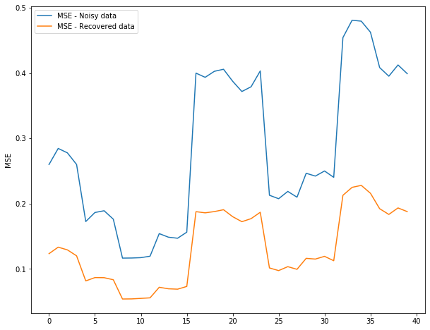
noisy_stat = []
recovered_stat = []

# print(len(train_set_3d))
for keys in list(train_set_3d.keys())[:40]:

    true_state = train_set_3d[keys]
    cov = np.cov(true_state.T)

    noise = np.random.multivariate_normal(mean = np.zeros(true_state.shape[1]), cov = cov, size = true_state.shape[0])
    noisy_observation = true_state + noise
    # print(keys)
    # print(noisy_observation.shape)
    filtered_onservation = KF_filter(noisy_observation)
    noisy_stat.append(mean_squared_error(true_state, noisy_observation))
    recovered_stat.append(mean_squared_error(true_state, filtered_onservation))
## Plotting the results (tentetive)
# complete this
fig = plt.figure(figsize=(10,8))
plt.plot(noisy_stat, label = 'MSE - Noisy data')
plt.plot(recovered_stat, label = 'MSE - Recovered data')
plt.ylabel('MSE')
plt.legend()
<matplotlib.legend.Legend at 0x7f5d272d7438>
References
[1] J. Martinez, R. Hossain, J. Romero, and J. J. Little, “A simple yet effective baseline for 3d human pose estimation,” in ICCV, 2017.
This wraps us the last assignment for Computer Vision course for Fall 19. The second part of the homework was small but did not click initially and required quite a few iterations for me but managed it in the end. (Though I don’t the question actually makes sense!)
Anyway, Peace!